Guest Post by David Churchward
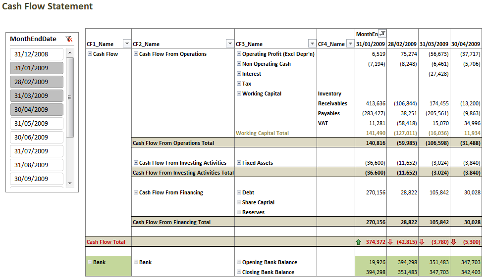
There’s few, if any, reports that I consider to be more important than the Cash Flow Statement. Every business needs one, probably above any other report. There’s numerous different versions of Cash Flow reports and, in reality, it can become a very personal thing to a company so I’m not going to propose to provide a one size fits all report. In addition, I’m not going to proclaim to provide an IAS7 – Cash Flow Statement (that’s International Accounting Standards) textbook report because this isn’t designed as an accountancy lesson (but, if you’re interested, the method I’ll show here relates to the Indirect Method in IAS7).
With that said, if you consider this post alongside Kasper’s excellent post Building a cash flow statement in PowerPivot using Dynamic Measures in DAX, you should have all the tools you need to produce any Cash Flow Statement that you require.
The Accountancy Bit (very quickly!)
Just before we start, a quick accountancy point to consider. Kasper’s approach considers cash payment and receipt transactions. My model uses all transactions in the general ledger with the exception of Bank transactions. On the basis that double entry exists (ie every transaction has an equal and opposite effect), all transactions that aren’t the bank transactions must equate to the same value. The reason we use the “other” side of the account is because this side of the transaction tells us what the cash transaction was for. As a result, we should simply be able to aggregate transactions into Cash Flow categories.
This seems quite straight forward. Unfortunately, there are a few exceptions that need to be handled. I’m only going to explain one which should give you the means to adjust for others.
Depreciation is purely an accounting adjustment. This has the effect of crediting the balance sheet and debiting the P&L. The effect of crediting the balance sheet has the effect of reducing the value that will be shown as Fixed Asset additions. We therefore net off the depreciation transaction as if it never happened and I’ll show this later in this post.
The Dataset
My dataset (FACT table) contains 3 columns:
- GL_Account– this is my general ledger code. Every transaction that forms the trial balance will carry a general ledger code and this tells us what the transaction was for.
- Month_End_Date – this date tells us the financial period to which the transaction relates. I would advise using the month end date of the financial period in which the transaction will be reported as I’m doing in this example. (or a period number as in Rob’s Greatest Formula In The World posts). It should be noted that a transaction date may not be in the same calendar period as the reporting date so care should be taken.
- Amount– this is the transaction value. Using normal accounting signage, this will be a positive value for debits and a negative value for credits.
My dataset contains all transactions processed on the system – this is PowerPivot, it can handle it – and this essentially forms the basis of the trial balance. If you have a lot of old data and don’t want to include it all, you could substitute historic data with opening balance values for each general ledger code. This simply aggregates a lot of old transactions into one balance (per general ledger code) for an opening balance date, whilst maintaining the overall integrity of a balanced trial balance and the associated values.
You may have a dataset that holds monthly values for each general ledger code as opposed to each individual transaction. This will work equally well although you won’t have the means to dissect the Cash Flow Statement by subset records such as customer or project.
If your data is held as monthly columns, it’s worth running an UNPIVOT. Whilst we could condition PowerPivot to work with individual values for each period, it’s more efficient to work with one value column with associated period dates held in another column.
Related Tables
I link my my FACT table to a GL_ACCOUNTS table on the GL_Account code. The GL_Accounts table provides details relating to the GL_Code such as account name and report heading codes. These heading codes, in turn, link through to a further GL_Headings table which holds cash flow report heading codes. This, in turn, links through to cash flow heading tables. It’s these headings that we will use on our Cash Flow Statement report.


You’ll notice that CF1 doesn’t link to any other tables. I’ll come onto that shortly.
General Ledger Account Mappings
The GL_Headings mapping is the critical element to this dataset. This provides all of the key relationships between a general ledger code and the Cash Flow Statement report heading that you want the account to be represented under.
GL_Headings Table

My GL_Accounts map through to my Heading_Code on this GL_Headings table. This table holds all of my key report headings and provides a useful grouping of accounts. For instance, all general ledger codes that relate to Sales will carry a Heading_Code of 1010.
These definitions are important. This is a one-off setup and you’ve probably done this indirectly in some way or another to drive any reports or Excel analysis that you’re currently doing (probably with VLOOKUP). This process simply affirms that mapping. Ideally, you would code these heading codes into your General Ledger account code setup and formulate the code allocation as part of the process to set up new general ledger accounts.
You’ll recall that I mentioned Depreciation earlier in this post. Whilst this is a P&L account (heading code 1045 in this example), I’m coding this to exactly the same place as Fixed Assets on the Balance Sheet (heading code 2010). This effectively eliminates the deprecation transactions. An alternative would be to filter out the accounts in question. You can do this, but be careful to ensure that those accounts net to zero.
Each of these codes map through to Cash Flow Statement heading tables. These heading tables can be whatever you need them to be, with headings and ordering assigned however you want your final report to be represented. The one’s I’m using are shown below.
CF2 – Cash Flow Statement Heading 2

This is my first grouping of headings. These align with the IAS7 headings for CF2 codes 1, 2 and 3 and basically split my Cash Flow Statement between Operations Activities, Investing Activities and Financing Activities.
There’s a fourth section called Bank. The Bank general ledger codes map through to this code and we eliminate them for the Cash Flow element of this report. However, we bring them back into action when we display the Bank Balances at the end of the report.
CF3 – Cash Flow Statement Heading 3

This is the next level of granularity on my report. The Bank general ledger codes don’t have any CF3 mapping and yet I’m carrying Opening and Closing Bank Balance codes on this heading set. I’ll come onto why that is a bit later. You’ll also notice that I’ve coded these headings with an Open_Bank and Close_Bank flag. We’ll use dynamic DAX measures later on to utilise these.
Note – there should NOT be any mapping of accounts to the CF3 codes 10 and 11 in this table (ie Open and Close Bank Balance). We’ll use these simply to drive a DAX measure later.
CF4 – Cash Flow Statement Heading 4
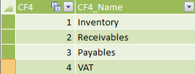
One element of my Cash Flow Statement will carry a further breakdown – Working Capital (although you can have more if you want). I’ve done this simply to provide an extra level of granularity, but you could decide to replace the Working Capital heading in CF3 with these headings and map accordingly.
I’ve got a few reasons for doing this:
- I like to show my Working Capital elements specifically – this targets the key operational balance sheet items that generally need to be tracked
- This helps to line up a future post!
CF1 – Cash Flow Statement Heading 1
You might, quite rightly, question why my ordering has gone to pot and I’m explaining CF1 last! Quite simply, this table sits out on it’s own because it simply drives report sections as opposed to being a mapped heading code. I’m going to show a Cash Flow section and then, below that, I’m going to show the effect on the bank balance. No relationships required.

And Now for the DAX – Cash Flow
I’ve got to be honest, this measure isn’t going to set the world alight. However, this goes to show how easy PowerPivot can be, especially if you condition your data properly. I’m creating a measure aptly called Cash_Flow
Cash_Flow
=CALCULATE(
SUM(FACT[Amount]),
CF2[CF2_Name]<>"BANK"
)*-1
This is a simple CALCULATE function which sums the [Amount] field on the FACT table with a simple filter set to ignore any GL_Accounts that have a CF2 category mapping of “BANK”.
You’ll notice that I multiply this by –1 to reverse the signage. In simple terms this is because of the double entry effect. We’re using the “other” side of the transaction which means that the sign convention is going to be back to front. This simply reverses that effect.
When I pull this measure onto my report together with the CF1,2,3,4 heading names, I get the following.
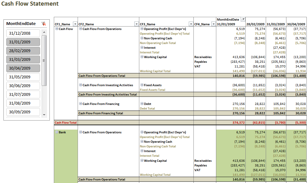
You might say that this is job done (especially if you remove CF1 heading from the report). This does give us a Cash Flow Statement. However, this doesn’t give my bank balances and, if I include my CF1 heading, my report is repeating the same data for both of the CF1_Name headings. This is understandable as CF1 is not linked to my FACT table in anyway. This is intentional (believe it or not!).
Bank Balances
I want to show opening and closing bank balances for the Bank section of my report and this is where it gets a bit more interesting. Let’s create a measure that calculates these balances and let’s call this measure Bank…
Bank
=IF(COUNTROWS(VALUES(CF3[CF3]))=1,
IF(VALUES(CF3[Close_Bank])=1,
CALCULATE(
SUM(FACT[Amount]),
ALL(CF3),
CF2[CF2_Name]="BANK",
FILTER(
ALL(Month_End_Dates[MonthEndDate]),
Month_End_Dates[MonthEndDate]<=
MAX(Month_End_Dates[MonthEndDate])
)
),
IF(VALUES(CF3[Open_Bank])=1,
CALCULATE(
SUM(FACT[Amount]),
ALL(CF3),
CF2[CF2_Name]="BANK",
FILTER(
ALL(Month_End_Dates[MonthEndDate]),
Month_End_Dates[MonthEndDate]<=
EOMONTH(MAX(Month_End_Dates[MonthEndDate]),-1)
)
),
BLANK()
)
)
)
We should be offering prizes for those of you would can instantly spot the GFITW elements!! Anyone would think that this had somehow been contrived! Believe me – it hasn’t. This is a concept that I use regularly and it’s a joy to see Rob explain it so well so I don’t have to!
So what is this doing? I’ll explain as clearly as I can, but it’s worth paying very close attention to Rob’s Greatest Formula In The World posts. I won’t re-iterate too much here.
- The first IF statement simply serves to provide an answer as to where I want the measure to be evaluated. I want an answer when my CF3_Heading is flagged as Open_Bank or Close_Bank.
- The second IF statement creates a value when my CF3_Heading [Close_Bank] is flagged. Where this is the case, the following happens:
- Sum the [Amount] Field
- Expand my dataset to all CF3 headings in order to release the dependency on the current CF3 heading being evaluated – ALL(CF3)
- Apply a filter to include all of my Bank general ledger codes – CF2[CF3_Name]=”BANK”
- Apply a further filter (FILTER) that:
- Removes the dependency on the MonthEndDate – ALL(Month_End_Dates[MonthEndDate])
- Apply a filter that includes all months that pre-date and include the reporting month – Month_End_Dates[MonthEndDate]<=MAX(Month_End_Dates[MonthEndDate]) – this is important because the transaction base for the month won’t give us the balance. We need to include ALL transactions that pre-date and include the reporting date.
- The third IF statement has a similar effect to the second IF statement, but it produces an opening balance and therefore the current reporting month has to be ignored. As a result, I want to sum all transactions where the date is less than or equal to my prior month date – Month_End_Dates[MonthEndDate]<=EOMONTH(MAX(Month_End_Dates[MonthEndDate]) ,-1)

Once again, we have the correct results but we’re getting values repeated for both CF1 headings.
Sorting Those CF1 Headings
We now have our two base measures. All we now need to do is evaluate when to use each one. Let’s create another measure called Cash_Flow_Statement.
Cash_Flow_Statement
=IF(COUNTROWS(VALUES(CF1[CF1]))=1,
IF(VALUES(CF1[CF1])=1,
[Cash_Flow],
[Bank]
)
)
This measure simply evaluates for CF1 headings and determines that if my CF1 Heading Code is 1 (ie Cash Flow) then use my [Cash_Flow] measure. Otherwise, use my [BANK] measure.
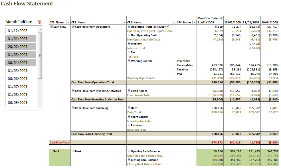
A bit of formatting and there you have it. You’re just about done. Or rather, you’re done if you think that’s enough. I, however, don’t like some of these totals and duplication of values in certain areas. There’s a way to deal with those totals but that’s a topic for a future post.
So what else can we do with this?
Just as a taster, here’s something that I like to call a Cash Flow Bridge. This could be a topic for a future post, but just to whet your appetite……
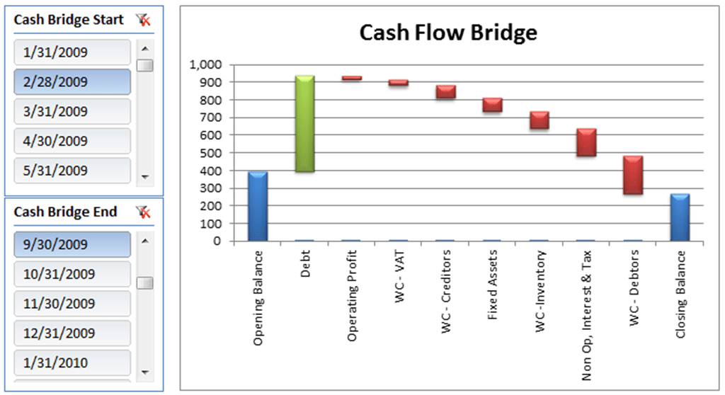
If there’s enough call for this, I’ll get this scheduled in for a future post. Neat eh!
Get in touch with a P3 team member