Grand Total Mania! (Totals at Top & Multiple Totals)

Let’s start 2014 with a bang…

I’ve been dying to write this post for awhile now.  Let’s say you want your grand totals to appear at the top of your pivot, like this:

Grand Totals at the TOP of the Pivot?  Yep, no problem.

Typically you’d want to do this when your pivot is really “tall” – lots of rows – and you don’t want to force people to scroll down in order to see the grand total.

Pivots do NOT let you display grand totals at the top of the pivot – only the bottom – so a frequent workaround is to write a formula in Excel itself that sums the whole column of the sheet.  Very clumsy, and damn near impossible when you have two fields on rows like above.

How DO You Do It, Then?

The trick is simple – add a dummy table to your Power Pivot data model:

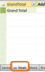
Dummy Table Named “Totals” with a Single Column
(Created via Linked Table)

And drag that dummy field to rows of the pivot, in top position…

Yielding…

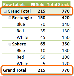
“Grand Total” Appears at Top AND Bottom, But the Top One is Our “Dummy” Field
(Which Just Happens to Have Just One Value – the Text Value “Grand Total”)

Now you just turn off Grand Totals on the Design ribbon…

Turn Off the “Real” Grand Totals

And now you just have it at the top!

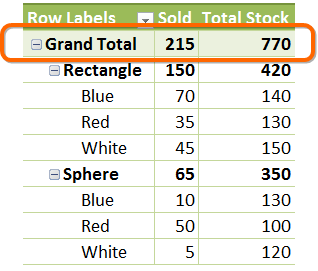
Voila!

Not Impressed?  OK, Try TWO DIFFERENT Grand Totals Then…

Hey, that trick above is actually pretty old – in fact I only learned of it from someone else, who found it on the MrExcel forums, and the trick was intended to be used with normal (non Power Pivot) pivots!

And yeah, a single calc column with a fixed value like =”Grand Total” does the trick – even in a normal pivot, yep.

A great trick.  A very Excel-style trick, as David Hager would say.  But can a normal pivot do THIS?

Whoa!  An Average-Based Grand Total AND a Sum-Based Grand Total in a Single Pivot??

Behind the Scenes…

Intrigued?  I hope so, because I absolutely love this one.  Of course, I am *the* precise kind of person who gets giggly over this sort of stuff, so maybe I’m alone, heh heh.

First I updated my dummy linked table to have a second column…

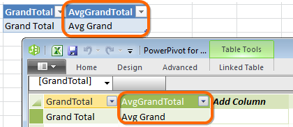
A Second Dummy Column.  Note the Absence of the Word “Total” From “Avg Grand.”

Then I wrote two “smart total” measures:

[Smart Sold] =

IF(ISFILTERED('Totals'[AvgGrandTotal]),
   [Avg Sold],
   [Sold]
  )

[Smart Stock] =

IF(ISFILTERED('Totals'[AvgGrandTotal]),
   [Avg Stock],
   [Total Stock]
  )

Added those to the pivot instead of the original measures [Sold] and [Total Stock], and added my new AvgGrandTotal dummy column to Rows (but NOT the GrandTotal dummy column in this case), yielding…

Getting Closer…  Just Need to Get Both Totals to the Bottom.

Next, on the Options ribbon tab, I go to field settings for my Avg Grand field…

Uncheck “Display Subtotals at the top of each group” checkbox for our dummy field

Yielding…

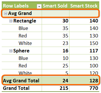
Then we hide the row of the worksheet that contains that “empty” subtotal from our dummy column…

Right Click Row Header, Choose Hide

And we’re done!

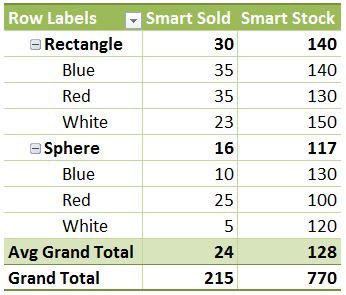
The End.

Download the Workbook!

I’ve made this workbook available for download here so you can conduct your own experiments