A common accounting task is to consolidate the financial results of subsidiary companies into combined results of a parent company. A parent company can have one or multiple subsidiaries. Each subsidiary can also have one or multiple subsidiaries beneath it. The relationships between parent companies and subsidiaries are often organized in a hierarchical structure.
In a single parent hierarchy, each child node has a single parent. In a multiple parent hierarchy, each child node can have either a single parent or two or more parents. In the single parent hierarchy diagram below, we can see that entities B and C have A as a parent, D and E have B as a parent, and F has C as a parent. The multiple parent hierarchy differs from the single parent hierarchy in that E has both B and C as a parent.

If we assume companies A, B, C, D, E, and F each have $100 of income the consolidated total would be as follows in the multiple parent scenario:
F: $100, E: $100, D: $100, C: $250 (100+100+50 assuming 50% ownership of E) B: $250, A: $ 600
For the single parent scenario, the totals would be the same except B would have $300 and C $200.
DAX has a hierarchy feature that is relatively straightforward to use for the single parent hierarchy scenario while a multiple parent scenario complicates things. The remainder of this writing will primarily focus on the latter.
The first time I built a hierarchy in DAX, everything appeared to be working well. However, as I checked the numbers, I realized that it was not handling the instances where a child node had multiple parents. I posted a question online asking if it was possible to create a hierarchy with multiple parents. The response I received was yes, it is possible……but it requires a many-to-many relationship to work correctly. I had previously read about many-to-many relationships online, and in Rob’s book, so I had a general idea of how to get started and thought that this problem would provide an excellent reason to explore it in more detail. I have an example workbook that you can download here to follow along
Before we can get to the task of creating a hierarchy, relationships, measures, and Pivot tables, we need three data sources:
- The hierarchy and ownership table
- A fact table with some transaction data
- A table with just a list of the unique hierarchy nodes (company names, etc…)
The first step is to create a table with the hierarchy nodes and ownership percentages. For this exercise, we will have 26 nodes or company names (1 each for A to Z). The first column is the Node ID. The second column is the parent Key. Nodes A, B, and C are top tier and do not have a parent. The nodes below A, B, and C will ultimately be consolidated into these three nodes. Looking at the fourth line, we can see that node A is the sole parent of node D.
Starting on lines 13 and 14, we can see that node M is duplicated in the Name column and that M has both D and G as a parent with each owning 50%. If M has an income of $100, $50 will flow up to both Node D and G respectively. The last four rows are for the four-way split of node Z. Node Z is owned 30% by T and U and 20% by W and X. Income for node Z will be split amongst these four nodes by these percentages.
Hierarchy nodes and ownership table
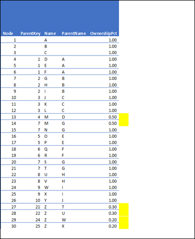
To summarize the table above, A, B, and C are top-level nodes and do not have a parent. M and Z have multiple parents while the remainder has a single parent. I should also note that when creating a node with multiple parents, the percentage total should add to 100%. Node M above is .5 + .5 and Z is .3+.3+.2+.2.
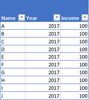
The second source of data needed is a fact table with transactional data. It will be kept simple for this exercise, and we will assume that all 26 entities from A to Z have an income of $100 in the year 2017 and $200 for the year 2018.
Partial Fact Table
The final data step is to create a table with a unique listing of the nodes.
Unique Nodes
| Name |
| A |
| B |
| C |
| D |
| E |
| F |
| G |
| H |
| I |
| J |
| K |
| L |
| M |
| N |
| O |
| P |
| Q |
| R |
| S |
| T |
| U |
| V |
| W |
| X |
| Y |
| Z |
Once the data is assembled, it can be loaded into the data model.
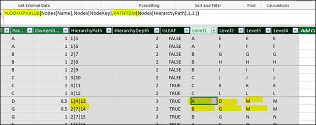
To complete the building of the hierarchy, some calculated columns will be added to the Nodes table. The DAX Path function is used to return the ID chain for the hierarchy path. It is a pipe-delimited list that has the parent ID for the chain. For node M on rows 13 and 14, the path is 1|4|13 and 2|7|14. As M has two parents, half of its income will flow up to nodes D and A while the other half will flow to nodes B and G
DAX PATH Function in the nodes table. The first five columns are raw data, and the last seven are calculated columns.
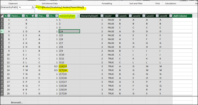
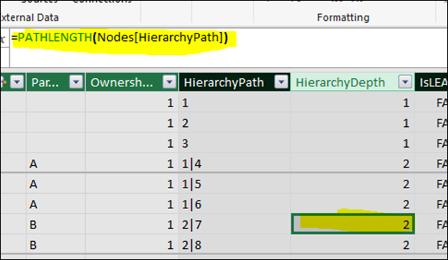
The DAX PATHLENGTH function returns the depth of the hierarchy chain. For this example, the maximum depth is four, so we will build four Levels (Level1,2,3, and 4) for the hierarchy.
For each of the four levels of the hierarchy, the DAX LOOKUPVALUE and PATHITEM functions are used to retrieve the corresponding entity name from the hierarchy path.
To create the hierarchy, while in the diagram view, click on the create hierarchy button in the top right corner and drag the fields to the bottom.
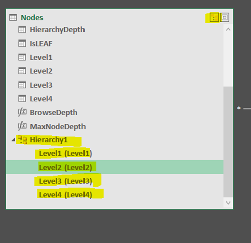
The hierarchy will appear in the pivot table field list.

The next step in the process is to set the relationships in the data model as follows:

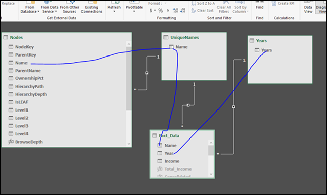
Next, we will need to create a few measures.
The first measure is straightforward in that it is only a SUM of the Income amount in the fact table.
Total_Fact_Income :=
SUM ( Fact_Data[Income] )
Our second measure [Total_Income] takes the income measure created above and wraps it inside a CALCULATE and passes the Nodes table as a filter. This is needed for the M2M to work.
Total_Income :=
CALCULATE ( [Total_Fact_income], Nodes )
I would recommend reading pages 220-228 of Rob’s latest book to get a better understanding of why it is done this way. The book provides a deeper dive into the subject and also discusses the subtle differences between PowerPivot and Power BI when dealing with M2M situations.
The third Measure is a SUM of the OwenershipPct column of the Nodes table.
PctOwnership :=
SUM ( Nodes[OwnershipPct] )
The Consolidated_Income measure is the primary measure that will be used for this example. It wraps the Total_Income measure in a SUMX function and multiplies by the ownership percentage.
Consolidated_Income :=
SUMX ( Nodes, [Total_Income] * [PctOwnership] )
Next, we can build a pivot table with the following selections:
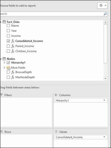
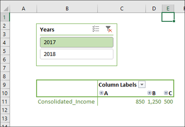
This pivot table displays the consolidated year 2017 income for the Top Level entities in the hierarchy. The consolidated total for A+B+C = 2,600.
With nodes A and B of the hierarchy expanded, we can see that 50% of the 2017 $ 100 income for Node M is allocated first to Node D and then to Node A and the other 50% flows up to G and B. The pivot table displays node M as a child of two different parents within the hierarchy.

The 30,30,20,20 allocation of Entity Z income to the four different parents is shown in the Pivot Table below.

There are two additional measures Parent_Income and Children_Income. I’m not certain that they function correctly, but they are my attempt to segregate the income of only the parent and the income of all children of the parent. The total of both should equal the consolidated income.

Microsoft’s platform is the world’s most fluid & powerful data toolset. Get the most out of it.
No one knows the Power BI ecosystem better than the folks who started the whole thing – us.
Let us guide your organization through the change required to become a data-oriented culture while squeezing every last drop* of value out of your Microsoft platform investment.
* – we reserve the right to substitute Olympic-sized swimming pools of value in place of “drops” at our discretion.
Get in touch with a P3 team member