
Data preparation has become so easy and potent in Excel and Power BI. The user experience of the Query Editor of Power BI and Excel (Power Query Add-In, or Get & Transform in Excel 2016) is extremely rewarding. It changes the crucial yet tedious and repetitive tasks into an exciting and even fun activity. Just as important, it’s a process which produces an automated pipeline for your ever-changing reporting requirements. Thanks to Power Query, the modern data wrangler can become a Self-Service ETL power house. As you move up on your journey to become a super data wrangler, it’s time to be aware of the most common mistakes you do in Power Query, and how to avoid them.
As you build your query using the Query Editor, each transformation step generates a formula, or a line of code. The sequence of formulas are generated as a script (In the language which is unofficially called “M”, or Power Query Formula Language) which allows Excel and Power BI to follow the transformation steps that you’ve defined in the user interface, and automate it whenever you refresh your report. While it’s not necessary to learn M to achieve 80% of your data transformations, it is extremely useful to be aware of it, and become confident enough to apply some lightweight touches to the formula and avoid common mistakes.
The common mistakes, which I also call Pitfalls, are almost rooted in the basic design of Power Query – by designing a system so robust and complete, they inadvertently left a few of these “pits” lurking. Only practice, awareness and education will take you out of the pitfalls, and train you to avoid them in the future.

The Root cause: Preview
So, what are those pitfalls, and why do we they exist? Data transformation in Power Query is always based on a snapshot of the data, and usually on a limited preview of it (e.g. 200 first rows). Each step you apply in the UI of the Query Editor is converted into a formula, which is heavily dependent on the preview/snapshot format . However, when real data starts deviating from the snapshot data, your queries will fail to refresh, or even worse, lead to incomplete or invalid data in your reports, which may ultimately lead to data-biased business decisions.
I’ve recently completed a series of blog posts here, that walk you through each of the 10 pitfalls, and I thought it would be best to wrap up this series here on p3adaptive.com. So let’s quickly go over the 10 Pitfalls in Power Query, and allow you to drill down to the original posts, whenever you are ready to learn it in more details, and avoid those pitfall.
Pitfall #1 – Your formula bar is inactive
If you don’t know what is the formula bar, that is alright. Open the Query Editor and check the Formula Bar checkbox in View tab. From now on, you will always have the formula bar visible. You can also enable the Formula Bar in the File tab –> Options & Settings –> Options –> Global –> Query Editor.
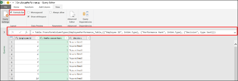
Why is it so important to activate the formula bar? The formula bar will be your best guide that warns you when you reach a pitfall. By getting to know what to look for in the formula bar, even without knowing the formula syntax itself, you will be able to understand the weaknesses of your queries, and to be better equipped to fix them when they fail.
Learn more here.
Pitfall #2 – Auto-generated Changed Types step
Whenever you import a table, or perform steps like split columns, an auto-generated step will decide the column types for you, to ease your data cleansing experience. But this step contains a formula that refers to all the column names. When one of the columns will be renamed or get deleted in your external data source, you will have a refresh error. It’s nice to get a free lunch. But free meals are not always nutritious.

The auto-generated Changed Type step is the #1 catalyst for refresh errors. You will do better by deleting this step, or tweak the formula to address only the crucial columns. Learn more here.
Pitfall #3 – Include vs. Exclude Filters
Whenever you apply a filter in the Query Editor, I encourage you to check the resulting formula bar and ensure the filter was applied on the correct values – Especially when you want to exclude values.
Let’s demonstrate it. Imagine, we would like to exclude all the rows with 1100 in Column 2 as highlighted below.
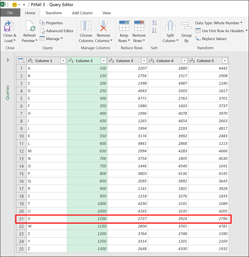
In the Query Editor, we click the filter control on the right side of Column 2’s header, and start searching for values that starts with “11”. Two values pop up: 1100 and 1105.
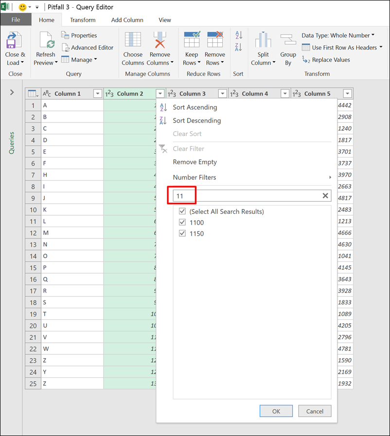
Now, we uncheck the value 1100, and click OK in the filter pane, expecting that it will filter out all the rows with 1100 in Column 2.
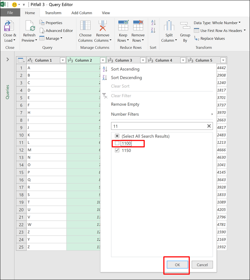
Surprisingly, we find out that the filter logic was automatically tuned to include only values of 1150 in Column 2. Here is where Pitfall #3 happens. We can easily miss the wrong logic, and have the wrong data being propagated into our reports.
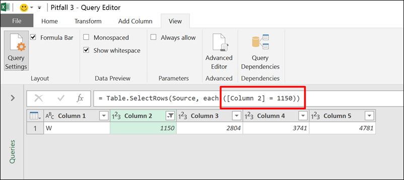
To fix the wrong logic, you can change the formula from:
[Column 2] = 1150
To:
[Column 2] <> 1100
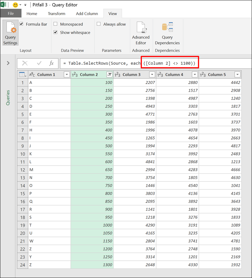
To learn more about the third pitfall, go here.
Interested in Learning How to Do this Kind of Thing?

Our New Online Power Query Course just launched this year. You’ll learn Power Query from the best in the business, two Excel MVPs Ken Puls and Miguel Escobar. We’ve included 7 Hours of Self-Paced Video over 31 Courses, with lots of example files, and a Digital Badge powered by Acclaim.
CLICK HERE to claim your spot.
Pitfall #4 – Column Reordering
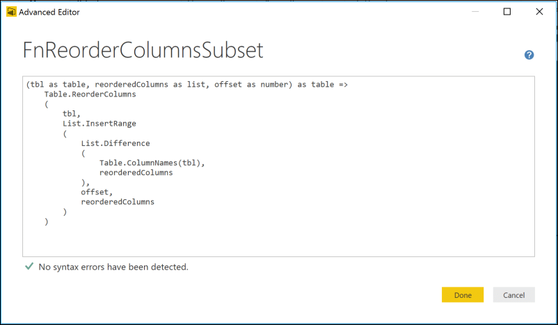
Reordering columns in the Query Editor is a tricky business. You often do it for ad-hoc debugging purposes, unaware of its weaknesses. The reordering creates a formula that refers to all the columns in the table. When one of the column is missing, the refresh will fail. To avoid this pitfall, and reorder a subset of the columns, you can apply an advanced query function. Learn more here.
Pitfall #5 – Removing and Selecting Column
Often times you remove unnecessary columns from your table using the Query Editor, instead of selecting the other columns you need to keep. To avoid refresh errors, when specific column names are missing, you can change the formula to refer to the column’s position instead of its name.
Instead of selecting the first two columns by explicitly refer to their names:
= Table.SelectColumns(Source,{“Column1”, “Column2”})
We can change the formula above to select the first two columns in a dynamic way, which will not fail when the column names change:
= Table.SelectColumns
(
Source,
List.FirstN(Table.ColumnNames(Source), 2)
)
Learn more here.
Pitfall #6 – Column Renaming
You import a table to Excel using the Query Editor, and find some cryptic column names, that call for an urgent rename. But hold on! Do you have a solid “Data Contract” with the owner of the external data source? Can you ensure that the columns will keep their current names? When you rename the columns in the Query Editor, you expose the query to a refresh failure that will surface when the column names in the external data source will change.
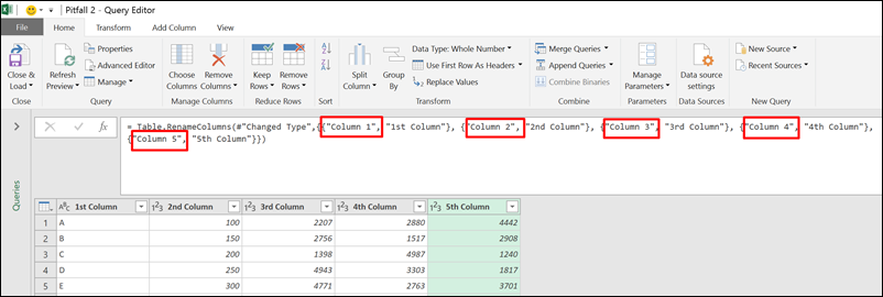
In this article you can learn how to apply the query function below to rename columns according to their position in the table:
(Source as table, ColumnNamesNew as list, Indices as list) =>
let
ColumnNamesOld = List.Transform( Indices, each Table.ColumnNames(Source){_} ),
ZippedList = List.Zip( { ColumnNamesOld, ColumnNamesNew } ),
#”Renamed Columns” = Table.RenameColumns( Source, ZippedList )
in
#”Renamed Columns”
Pitfall #7 – Split Columns By Delimiter
This pitfall is one of my favorites. When you split columns by a delimiter, the Query Editor creates new columns to accommodate the split values
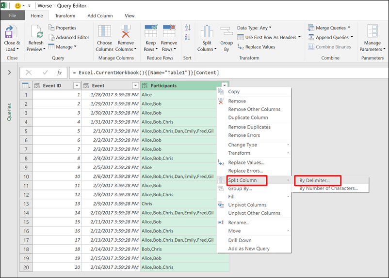
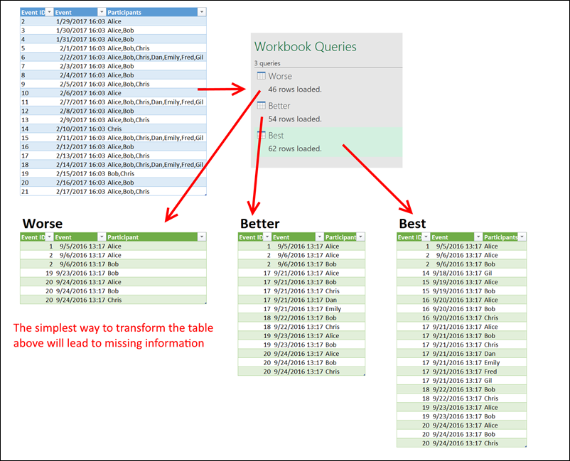
Unfortunately, the number of new columns, that is needed for the split, is decided during the evaluation of the preview data. When the external data will change, lots of crucial information may get lost. In the screenshot below, you can see an example of a table with participants in events. Each event is represented in a single row, with comma-separated participants in the third column. When I created the query, there were no more than three participants in an event. As a result, the query split the column Participants into three columns. Later, when the data changed, I completely lost the fourth participant end beyond in events with more than 3 participants. Read more here to find how to build the Better and Best queries.
Pitfall #8 – Merge Columns
The reverse transformation of Split Column is less popular, but is quite handy, and simple to use. I often use it when I need to unpivot multiple columns in a nested table (For unpivot of nested table, read more here).
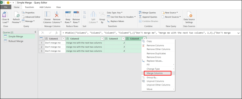
The pitfall lies in the fact that the merge step creates a complicated formula which will fail when the column names will change.

In case you need to merge columns according to their position, and not by their names, you can follow this article to learn how.
Pitfall #9 – Expand Table Columns
Expand Table Column is a common transformation step that you can take advantage of when you merge between two queries, or import JSON or XML datasets. The Expand Table Column step occurs when you click on the highlighted button:

Expanding the Table columns activates the expand pane, which allows you to select the columns to expand. Unfortunately, you need to define the columns, and these columns are hard-coded into the formula.
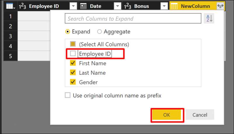
Imagine we want to expand all the columns except Employee ID. When we uncheck Employee ID in the pane above, we get the following formula:
= Table.ExpandTableColumn(#”Merged Queries”, “NewColumn”, {“First Name”, “Last Name”, “Gender”}, {“First Name”, “Last Name”, “Gender”})
The columns First Name, Last Name and Gender are hard-coded, and this is our pitfall. If we need to extract other columns which are not presented in the preview, can we extract them dynamically? The answer is yes.
= Table.ExpandTableColumn(#”Merged Queries”, “NewColumn”, List.Difference(Table.ColumnNames(Employees), {“Employee ID”}))
Learn more here.
Pitfall #10 – Remove Duplicates and Lookup Tables
Last but not least, the tenth pitfall explains how to effectively create lookup table using the Remove Duplicates step in the Query Editor. How many times, did you create a look table using the Remove Duplicates in Power Query? As a lookup table requires a One-To-Many relationship with the relevant column in your fact table, it is imperative that you keep your values unique. Apparently, and this is why the tenth pitfall is so common, the Query engine and Power Pivot don’t share the same logic with regards to unique values. So removing duplicates is not sufficient to avoid the pitfall and avoid refresh error. Read more here.
Conclusions
Avoiding the ten pitfalls is a crucial step in becoming a successful data wrangler – One that can deliver production-ready robust queries. You can now follow the Pitfalls series whenever you encounter refresh errors or unexpected results in one of the 9 transformations we have described in this series. Creating robust queries that won’t fail you on the next refresh, can be easily achieved. And, you don’t really need to master M to avoid the pitfalls, and gain robust queries.
Hope you enjoy this series. Looking forward to learning about other pitfalls you have encountered.
Get in touch with a P3 team member