Restructure Your Data Table for Improved Compression

I was relaxing during my vacation thinking some more about column compression in Power Pivot.  One of the main things to know about compression is that a high level of cardinality is your main enemy (ie a large number of unique values will mean poor compression).  I started to think about how I could reduce the cardinality of one or more columns in a large data table I use for a client.  This blog covers the process I went through to test a couple of concepts – warts and all – including a simple error I made during the early testing for this blog post.  I think you can sometimes learn more when you make and then find a mistake, hence I have kept the error I made in this post for others to see along with the fix.  What I think is interesting about this is the process of discovery to find the problem.

The data table I used for my test is a typical sales table, and it includes line level extended cost, line level extended sell, quantity of cases sold among other things.  With this data structure in mind, there were 2 opportunities that immediately came to me.

Swap out Extended Price for Margin %.

The first idea I had was to swap out one of the value columns (either extended cost or extended sell) with a margin % column.  Given it is very common for resale businesses to work with a fixed range of margin %, this should reduce the number of unique values in one column while still allowing the recalculation of the missing data from the other column. 

Swap out Extended Values with Price per Case

The second idea was to recalculate the 2 extended columns with prices per case.  Eg, think about a typical reseller situation where products are sold for (say) $1.00 per unit.  A customer can buy any number of units and for each variation in quantity there will be a different unique value of the sales value resulting in an increase in the cardinality of the column.  Swapping the extended column with the price per case should reduce the cardinality and hence could improve the column compression.

But what about the DAX?

The big potential issue with both of these alternate approaches is that you can no longer use simple aggregators like SUM() in your DAX formulas.  Once you change the data structure to one of those above, you will need to start to use SUMX ( ) instead of SUM( ).  SUMX is an iterator and this could have negative impacts on performance on a big data table – read on to see what happened in my testing.

It’s Important to use Real Data for this Test

In my last blog post I used random numbers for my testing.  That was fine for that test scenario however in this case I really need to use real data.  Everyone’s data is different, and a test like this is pointless unless you use real data.  So for this test I loaded up 2 years of real data totalling 27 million rows in the sales table.  The file size on disk is 264MB – perfect for testing and a genuine candidate to reduce the file size.

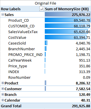
The first thing I did was load up the data into a new Power Pivot workbook exactly as it is currently used, including an extended cost, extended sell and a qty column (CasesSold).  I inspected the size of the columns using Scott’s enhanced VBA code (originally written by Kasper de Jonge).

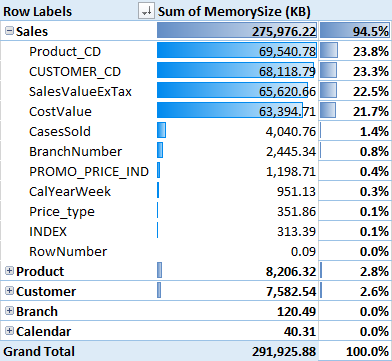
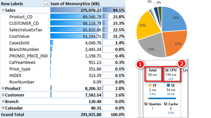
As you can see above, the SalesValueExTax column takes up 22.5% of the total memory, and the cost value column uses slightly less at 21.7%.

My regular DAX formulas using this data structure look like this – very simple indeed.

Total Cost :=SUM(Sales[CostValue])

Total Sales := SUM(Sales[SalesValueExTax])

Total Margin % := DIVIDE([Total Sales] – [Total Cost] , [Total Sales])

Test 1 – Replace the SalesValueExTax with Margin %.

I could swap out either the extended cost or the extended sell column for this exercise, but I decided to remove the sell column because it is larger (see how useful the “what’s eating my memory tool is”).    I wrote a SQL Query to modify the data on import as follows (note the rounding to keep the margin decimal places to 1 and hence keep the cardinality low.   Three decimal places = 1 decimal point for a percentage).  This level of accuracy is exactly what is used in real life, so there should be no issues with the rounding:

SELECT  s.[CalYearWeek]
,s.[BranchNumber]
,s.[CUSTOMER_CD]
,s.[PRODUCT_CD]
,s.[Price_type]
,s.[PROMO_PRICE_IND]
,round((s.[SalesValueExTax] – s.[CostValue]) / s.[CostValue],3) as [Margin %]
,s.[CostValue]
,s.[CasesSold]

FROM [dbo].[tblSales] as s  WHERE ([CalYearWeek] >= 1401)

This single change reduced the file size on disk from 264MB to 245MB – a reduction of around 7%.  Not too bad.  Of course once this change is made, I needed to change the DAX.   [Total Cost] stays the same but Total Sales needs to change and use an iterator as follows:

Total Cost :=SUM(Sales[CostValue])

Total Sales := SUMX(Sales,DIVIDE([Total Cost] , 1 – Sales[Margin %]))

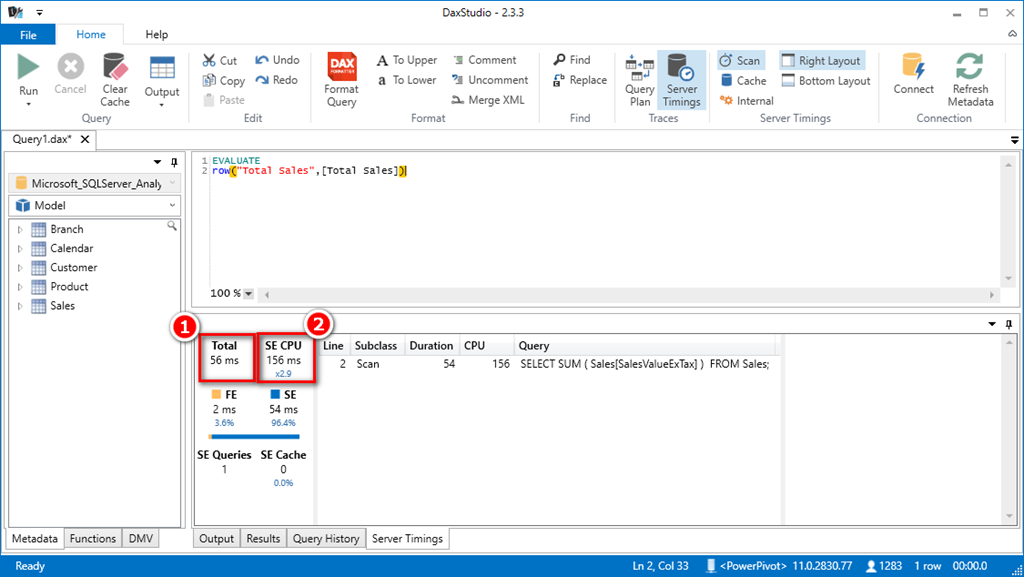
The big problem with this approach is the need to use SUMX instead of SUM to do the calculation.  Iterating over a table with 27 M rows is going to be relatively slow.  To test this objectively, I loaded up DaxStudio and used the Server Timings feature to see how long it took to calculate the [Total Sales] on both workbooks.

With the original data model, it took a total of 56 milliseconds (ms) as shown in 1 below.  Also note how the Storage Engine leveraged multiple cores for its part of the process using 156 ms in total CPU time effectively across 2.9 processors (shown in 2 below).

Then I tested with the second workbook requiring the use of SUMX.  I was not expecting the same level of performance however unfortunately the response time was really bad – 253 seconds as shown below.  I was expecting a lesser performance, but not that bad!  Something must be wrong.

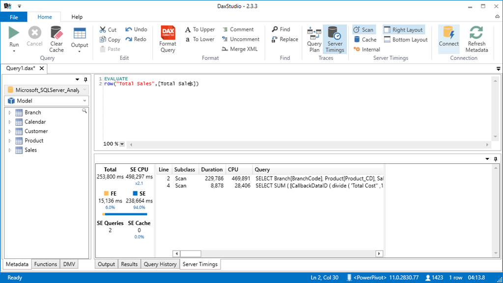
On the face of it, this looks like an unworkable solution.  However read on to see my journey of discovery as all is not lost just yet.  I made a simple mistake here and that will become clear shortly (if you haven’t already spotted it).

Test 2 – Swap out the Extended Columns for “Per Unit” Values

Just like the first test, I used SQL to change the structure of the data I loaded into Power Pivot.  Here is what the new Query looks like (note the rounding to keep the decimal length to 2 which keeps the cardinality low).

SELECT  s.[CalYearWeek]
,s.[BranchNumber]
,s.[CUSTOMER_CD]
,s.[PRODUCT_CD]
,s.[Price_type]
,s.[PROMO_PRICE_IND]
,round(s.SalesValueExTax / CasesSold,2) as SellPerCase
,round(s.[CostValue] / CasesSold,2) as CostPerCase
,s.[CasesSold]

FROM [dbo].[tblSummaryCWDConsolidated] as s  WHERE ([CalYearWeek] >= 1401)

The size of the file stored on disk went down from 264 MB to 247 MB, a reduction of 6.4%.

The new DAX formula will be

Total Sales : = SUMX(Sales,Sales[SellPerCase] * Sales[CasesSold])

This time the performance as measured by DAX studio is actually pretty reasonable as shown below.

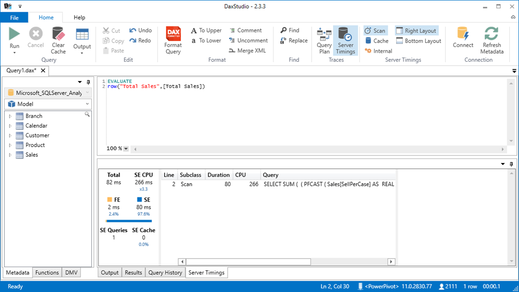
It is still slower than the original 56 ms – almost 50% slower at 82 ms – but this is still more than satisfactory for production use.

What is going on here?

So now I was feeling really uncomfortable – why was this second test so much better than the first test?  The anatomy of the two SUMX formulas is not too dissimilar – ie they both iterate over the sales table and do a calculation – so what is going on here?  Why is the first one so bad?!  When I looked at the actual query in DAX Studio I could see that Power Pivot was treating these 2 queries from test 1 and test 2 completely differently as shown below.

Test 1 – Very complex query with joins to the lookup tables

Note the complex highlighted query from DAX studio below, and also note there are 2 separate queries – only the first one is shown here.

Test 2 – Very simple query with no joins to the lookup tables.

Note how simple this second query is compared to the first.

So then I started to get curious – what was it about Test 1 – the Margin % example that meant the query was so complex.  The 2 things I noticed were

1.  I was using the DIVIDE function in the first test.

2.  I am using a measure inside the SUMX in the first test.

Edit (thanks to comments from Greg below): The measure inside SUMX has an implicit CALCULATE wrapped around the formula.  This forces context transition and this causes the formula to perform the way it does.  I rewrote the formula and replaced the measure.  The code then became.

Total Sales := SUMX(Sales,DIVIDE(Sales[CostValue] , 1 – Sales[Margin %]))

Once I made this change and re-ran the test in DAX Studio, I got a much better result.

This time it only took 638 ms in total.  A lot slower than the SUM version but still workable in many instances.  The report it self was snappy and produced sub second refresh on typical pivot tables – so all good.

Test 3 – Combine both concepts together

Finally I combined both concepts together, converting the extended cost to a cost per case and also swapping out the extended sell with a margin column.  The formulas needed to change slightly, and they were slightly less performant than the previous test – but still sub second.  The real spreadsheet continued to perform sub second on typical reports.

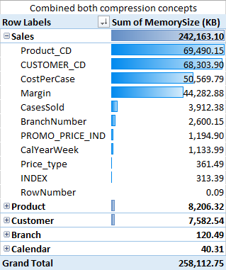
With both of these concepts combined, the file size was reduced from the original 264 MB to 238 MB, a reduction of almost 10%.  You can see where the space savings have come from by comparing the before and after column sizes in the 2 tables below.  The SalesValueExTax column (65MB) was replaced with the Margin column (44MB) and the CostValue column (63MB) was replaced with the CostPerCase column (50MB).

And here are the corresponding distinct count of values for each of the columns

Lessons from the Experience

1. You can get reasonable file size reductions if you think about your data structure and try to find ways to reduce cardinality.
2. The “What’s eating my Memory” tool is invaluable in helping you understand where to invest your effort.
3. DAX Studio is a very powerful tool that will help you understand where bottle necks are created and can help you improve your DAX Formulas so they are more efficient.
4. SUMX is an iterator, but it can be fast enough for production use as long as you write your formulas correctly.

Of course this test was done on my data, and the results on your data may/will be different.  But hopefully this article will give you some ideas about what to look for and how to go about testing your ideas.