
Guest Post by David Churchward
PART 1 and PART 2 of this series on Profit and Loss posts covered the basic layout of the P&L together with some time intelligence and filtering to display relevant numbers to cover actual, budget and prior year for both a selected period and the equivalent year to date. This was all based around the core measure referred to as Cascade_Value_All.
In this post, I’ll go on to refine this report further by adding Return On Sales (ROS) percentages and variance calculations as well as tune up the appearance of the report.
Return on Sales (ROS)
Return on Sales (or ROS for short) is the percentage that a number on our report represents as a function of the equivalent sales value. Most people will be familiar with the term Gross Margin Percentage and this is one type of ROS. Gross Margin percentage is a function of gross margin value divided by sales value. This is often dissected by individual product lines as the gross margin values are analysed by the same product categories as sales. Operating Profit Percentage is another ROS measurement but this is not normally sub analysed (although it can be if your dataset lends itself to that approach).
You’ve probably deduced that the financial calculation is therefore:
ROS %= Analysed Value / Equivalent Sales Value * 100
We’ve already got the value to be analysed in our model. This is the Cascade_Value set of measures. Therefore, we simply need to create the Equivalent Sales Value measure. I’ve called this measure Sales_Compare.
Calculating the Equivalent Sales Value – Sales Compare
In PART 2, we ended up with 6 measures (Cascade_Month_Actual, Cascade_Month_Budget, Cascade_Month_Actual_PY and the equivalents for YTD). We can use these measures as the basis for for a new set of Sales_Compare measures. I’ll run this example on the Cascade_Month_Actual measure. The same methodology applies for the other Sales Compare measures that we’ll use for each of our final report headings.
My Cascade_Month_Actual carefully sums the underlying dataset for each of my report headings (Report Heading 1 contains my main groups and Report Heading 2 contains my sub groups). I need to maintain my Report Heading 2 categorisation but remove the link from my Report Heading 1 categorisation. This is done using an ALL() function within a CALCULATE function.
SalesComp_Month_Actual_Interim
=CALCULATE(
[Cascade_Month_Actual],
ALL(DIM_Heading1),
DIM_Heading1[Heading1_Name]=”Sales”
)
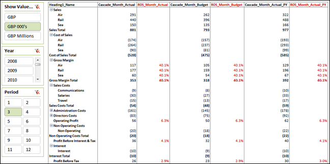
You’ll notice that I use my Cascade_Month_Actual measure, remove any association that it may have with Heading 1 and then direct it to filter the measure based on Heading 1 being equal to “Sales”. This way, I essentially repeat my sales value in each section of my P&L report.
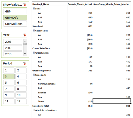
It should be noted that this is an interim calculation. It doesn’t necessarily make sense as it stands in the report above, but it will prove useful in further calculations. Having said that, I would prefer to only see the values in the sections where I want to display ROS percentages. In order to do this, I need to tell my dataset where I want to see ROS percentages displayed. To do this, I go to my DIM_Heading1 table and create a field where I can mark the headings where I want ROS calculations to be performed. I’ve called this field Heading1_PCT and mark the headings where I want to drive this calculation with a 1.
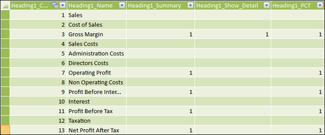
I can now reference the Heading1_PCT field to determine when the Sales Compare measure should return a result. We’ll call this measure SalesComp_Month_Actual.
SalesComp_Month_Actual
= IF(
COUNTROWS(VALUES(DIM_Heading1[Heading1_PCT]))=1,
IF(VALUES(DIM_Heading1[Heading1_PCT])=1,
CALCULATE(
[Cascade_Month_Actual],
ALL(DIM_Heading1),
DIM_Heading1[Heading1_Name]=”Sales”
),
BLANK()
),
BLANK()
)
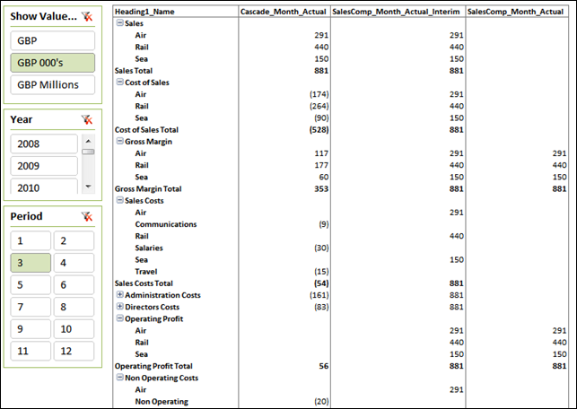
The calculate function is exactly as per our previous measure but I’m only running the calculate function when Heading1_PCT is equal to 1. I can only conduct this evaluation when I only have 1 value for Heading1_PCT so I have to use COUNTROWS and VALUES to determine this.
Calculating ROS
We now have the two key measures to derive our ROS being Cascade_Month_Actual and SalesComp_Month_Actual. I could simply divide one by the other surely. Essentially, that is correct, but as explained at length in Profit & Loss – The Art of Cascading Subtotals, we need the measure to behave slightly differently in different sections of the report. You’ll notice above that I have SalesComp_Month_Actual detail values for Operating Profit and Gross Margin. I only want my ROS calculation to evaluate at the total level for Operating Profit but at the detail level for Gross Margin. I can therefore use the evaluation that I used in my Cascade_Value_All measure and join it up with my simple division.
ROS_Month_Actual
= IF(
MAX(DIM_Heading1[Heading1_Summary]) = 1
&&(MAX(DIM_Heading1[Heading1_Show_Detail]) = 1
||COUNTROWS(VALUES(DIM_Heading2[Heading2_Name])) > 1
),
[Cascade_Month_Actual]/[SalesComp_Month_Actual],
blank()
)
My logical test is exactly the same as the one we saw in Cascade_Value_All in Profit & Loss – The Art of Cascading Subtotals. After that, it’s a simply division.
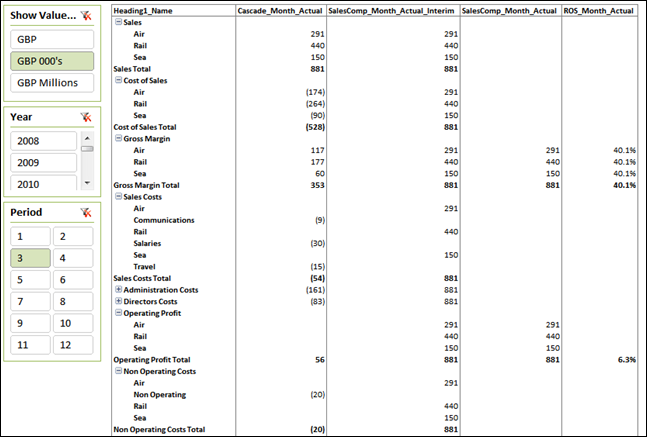
This same method is used for each associated column measure that we wish to calculate an ROS for. If I also remove my interim measures and apply some formatting, I get the layout below for month actual, month budget and month prior year. I should take this opportunity to apologise for not having been very inventive when I made this dataset up having used a flat set of percentages!
Variances
To complete the picture, we need to add some variance calculations. Because of the way that we’ve built up our measures, this is now very simple. Our actual versus budget variance is
Variance_Month_AvB
= [Cascade_Month_Actual] – [Cascade_Month_Budget]
I’m not going to insult your intelligence by writing out the equivalent for actual versus prior year.
Tidy Up
My report is going to display data for a selected month and the year to date position for that month. I prefer to split the two sections with a blank column. I don’t think we’re going to register on Rob’s spicy scale for this one!
Blank = BLANK()
Headings and CUBEVALUE
To give my measure names meaning and to allow for their careful use, they’ve become somewhat ugly. You can of course provide a title for the column that is a lot more user friendly. However, I prefer to write my own because I can make it look tidier and, more importantly, I can reference the period that has been selected on my slicer.
I use an Excel formula in my heading that uses a CUBEVALUE function to call the period number that I’ve selected. You could also do the same with year selections.
=”Period – “&CUBEVALUE(“PowerPivot Data”,”[Measures].[Maximum of Period]”,Slicer_Period)
This appends the period number onto the text “Period – “ by referencing the MAX value for Period when brought into the context of my slicer called Slicer_Period. I do the same for YTD, add a few more headings to describe the type of data and then hide my pivot table headings!
When It All Comes Together
When you put all of these elements together (PART1, PART2, Sales Compare, ROS, Variances, Blank and Headings) you get something like this….
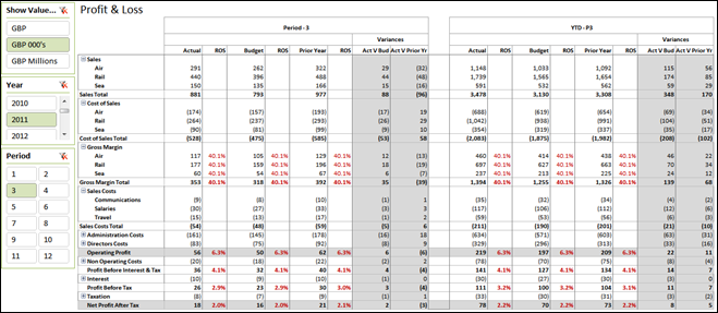
You can DOWNLOAD THE WORKBOOK HERE
Get in touch with a P3 team member