Implementing a Dynamic Top X via slicers in Excel 2013 using DAX queries and Excel Macros

Our First Post on Excel 2013 Beta!

Guest post by…  Kasper de Jonge!

Notes from Rob:  yes, THAT Kasper de Jonge.  We haven’t seen him around here much, ever since he took over the Rob Collie Chair at Microsoft.  (As it happens, “de Jonge” loosely translated from Dutch means “of missing in action from this blog.”  Seriously.  You can look it up.)

1) Excel 2013 public preview (aka beta) is out, which means that now we’re not only playing around with PowerPivot V2 and Power View V1, but now we have another new set of toys to take for a spin.  I am literally running out of computers – I’m now running five in my office.  Kasper is here to talk about Excel 2013.

2) I’ve been blessed with a number of great guest posts in a row, and there’s already one more queued up from Colin.  This has given me time to seclude myself in the workshop and work up something truly frightening in nature that I will spring on you sometime next week.  But in the meantime, I hand the microphone to an old friend.

Back to Kasper…

Inspired by all the great blog posts on doing a Dynamic Top X reports on P3 Adaptive I decided to try solving it using Excel 2013. As you might have heard Excel 2013 Preview has been released this week, check this blog post to read more about it.

The trick that I am going to use is based on my other blog post that I created earlier: Implementing histograms in Excel 2013 using DAX query tables and PowerPivot. The beginning is the same so I reuse parts of that blog post in this blog.

In this case we want to get the top X products by sum of salesamount  sliced by year (using adventureworks). To get started I import the data into Excel. As you might know you no longer need to separately install PowerPivot. Excel 2013 now by default contains our xVelocity in-memory engine and the PowerPivot add-in when you install Excel. When you import data from sources to Excel they will be available in our xVelocity in-memory engine.

I start by opening Excel 2013, go to the data tab and import from SQL Server:

I connect to the database server and database and select the tables DimProduct, DimDate and FactInternetSales:

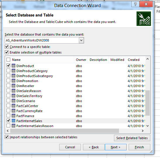
Key here is to select the checkbox “Enable selection of multiple tables”. As soon as you select that the tables are imported into the xVelocity in-memory engine. Press Finish and the importing starts.

When the import is completed you can select what you want to do with the data, I selected pivottable:

Now I get the pivotable:

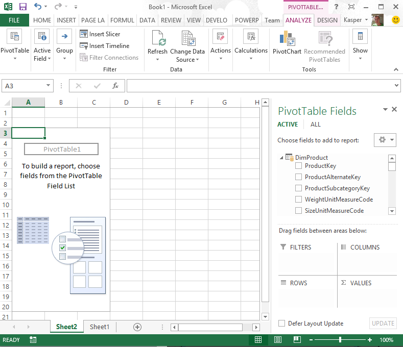
I am not actually going to use the pivottable, I need a way to get the top selling products by Sum of salesAmount. First thing that I want to do is create a Sum of SalesAmount measure using the PowerPivot Add-in. With Excel 2013 you will get the PowerPivot add-in together with Excel, all you need to do is enable it.

Click on File, Options, Select Add-ins and Manage Com Add-ins. Press Go.

Now select PowerPivot and press ok:

Now notice that the PowerPivot tab is available in the ribbon, and click on Manage, to manage the model

Select the FactInternetSales table, and the SalesAmount column, click AutoSum on the ribbon.

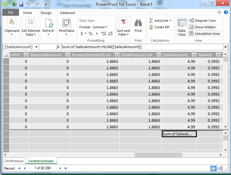
This will create the measure Sum of SalesAmount in the model.

Next up is creating a table that will give us the top 10 Products by Sum of SalesAmount.

There is not an easy way to get this using a PivotTable (See the blog posts by Colin to see how you can do it). I am going to use a new Excel feature called DAX Query table, this is a hidden feature in Excel 2013 but very very useful! Lets go back to Excel, select the data tab, click on Existing connections and select Tables:

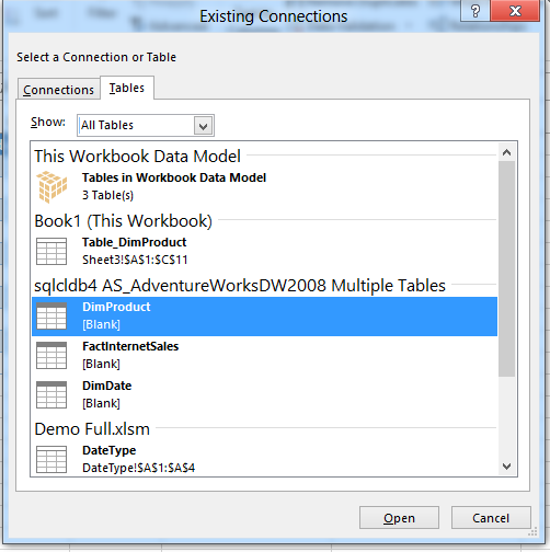
Double click on DimProduct and select Table and New worksheet:

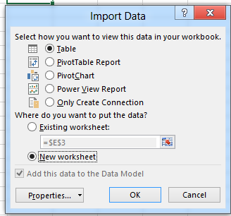
This will add the table to the Excel worksheet as a Excel table:

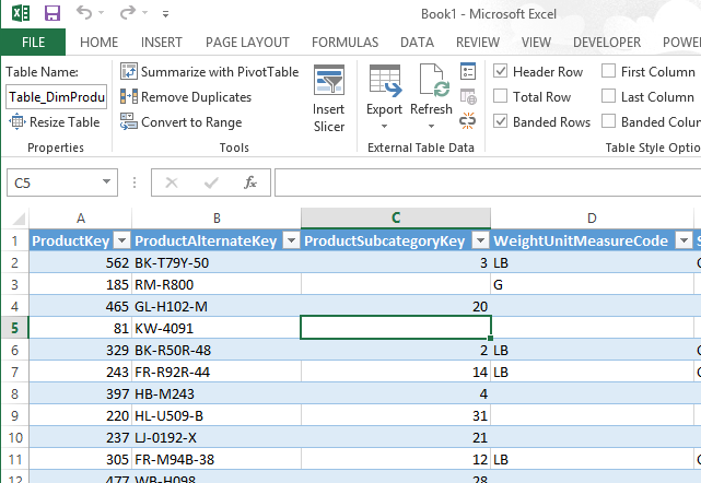
Now this is where the fun starts. Right mouse click on the table, Select Table, Select Edit DAX (ow yes !).

This will open a hidden away Excel dialog without any features like autocomplete and such:

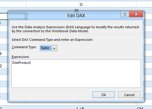
But it will allow us to create a table based on a DAX query that points to the underlying Model. What I have done is create a DAX Query that will give us the Top 10 products filtered by a year and pasted it in the Expression field. When you use a DAX query you need to change the command to type to DAX.

This is the query that will give us the top 10 products by Sum of SalesAmount filtered by Year.:

EVALUATE
ADDCOLUMNS(
TOPN(10,
FILTER(CROSSJOIN(VALUES(DimProduct[Englishproductname])
,VALUES(DimDate[CalendarYear]))
, DimDate[CalendarYear] = 2003
&& [Sum of SalesAmount] > 0
)
, [Sum of SalesAmount])
,”Sales”, [Sum of SalesAmount])
ORDER BY [Sum of SalesAmount] DESC

This results in the following table:

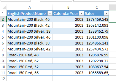
Since DAX queries don’t give formatted results back (unlike MDX) we need to format Sales ourselves using Excel formatting.  Now here comes a interesting question, how do we get this to react to input from outside? There is no way to create slicers that are connected to table, so we need to find a way to work around this.

Since this is a native Excel feature now we can actually program these object using an Excel Macro and that is what we are going to do. But first we just add two slicers to the workbook. One for the years and the other one for the TOP X that I want the user to select from.

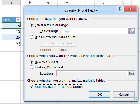
I created a small table that contains the top X values in Excel and pushed that to the model. To do that I selected the table, click insert on the ribbon, Pivottable and select “Add this data to the Data Model”:

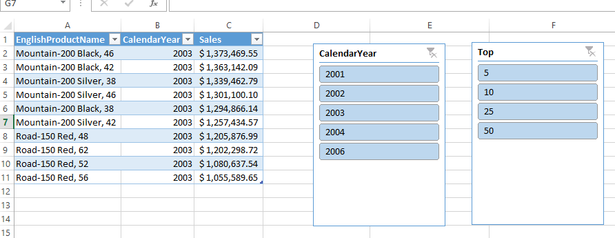
After that I created both slicers, both based on model tables, click Insert, Slicer and select “Data Model” and double click on Tables in Workbook Data Model

Now how do we get the query we used in the table to change based on the slicer selection? First I changed the name of the Table to “ProdTable” and Sheet to “TopProducts”.

Next I wrote a Marco that will get the values from the Slicers and create a DAX query on the fly and refresh the connection to update the table. I added a procedure to the code for the sheet:

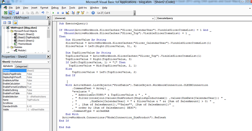
By the way I learned this by starting the Marco recording and start clicking in Excel 🙂 just try it, you’ll love it.

This is the Macro I wrote to change the DAX query of the Table based on the slicer values and refresh the table (disclaimer: it will not be foolproof nor perfect code):

Sub ExecuteQuery()

‘Make sure only one value is selected in both slicers
If UBound(ActiveWorkbook.SlicerCaches(“Slicer_CalendarYear”).VisibleSlicerItemsList) = 1 And _
UBound(ActiveWorkbook.SlicerCaches(“Slicer_Top”).VisibleSlicerItemsList) = 1 _
Then
‘ Get the slicer values from Slicer CalendarYear
Dim SlicerValue As String
SlicerValue = ActiveWorkbook.SlicerCaches(“Slicer_CalendarYear”).VisibleSlicerItemsList(1)
SlicerValue = Left(Right(SlicerValue, 5), 4)
‘ Get the slicer values from Slicer Top
Dim TopSlicerValue As String
TopSlicerValue = ActiveWorkbook.SlicerCaches(“Slicer_Top”).VisibleSlicerItemsList(1)
TopSlicerValue = Right(TopSlicerValue, 3)
If Left(TopSlicerValue, 1) = “[” Then
TopSlicerValue = Mid(TopSlicerValue, 2, 1)
Else
TopSlicerValue = Left(TopSlicerValue, 2)
End If

‘Load the new DAX query in the table ProdTable
With ActiveSheet.ListObjects(“ProdTable”).TableObject.WorkbookConnection.OLEDBConnection
.CommandText = Array( _
“evaluate ” _
, ” Addcolumns(TOPN(” & TopSlicerValue & ” , ” _
, ” filter(crossjoin(values(DimProduct[Englishproductname]) ,values(DimDate[CalendarYear])) ” _
, ” ,DimDate[CalendarYear] = ” & SlicerValue & ” && [Sum of SalesAmount] > 0) ” _
, ” , [Sum of SalesAmount]),””Sales””, [Sum of SalesAmount])” _
, ” order by [Sum of SalesAmount] DESC”)
.CommandType = xlCmdDAX
End With
‘Refresh the connection (might be hard to find the connection name.
‘If you cant find it use Macro recording
ActiveWorkbook.Connections(“ModelConnection_DimProduct”).Refresh
End If

End Sub

Unfortunately there is no way to react to a slicer click event or something like that. I decided to use a worksheet_change event, now here is another issue. How to get a worksheet to change on a slicer click ?

I decided to create a hidden pivottable that I connect up to the slicers so clicking would change the pivottable and hide it behind the slicers:

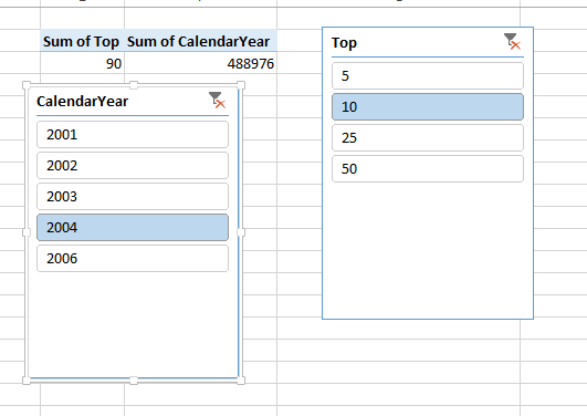
Now we end up with this worksheet:

Last thing that we need to do is connect the worksheet change event to the procedure we created. I created a procedure that I also added to the code part of the worksheet, it checks if something changes on the TopProducts sheet we execute the refresh of the pivottable.

Private Sub Worksheet_Change(ByVal Target As Range)
If ActiveSheet.Name = “TopProducts” Then
Call ExecuteQuery

End If

End Sub

And that is all there is to it . This allows us to get a dynamic top x based on slicers, now ofcourse you can do whatever you want with the results, use them in a graph and so on.

Hope you enjoyed Excel 2013 and all the new features that it brings, like Marco’s to the underlying Model and DAX query tables right in Excel !