Guest Post by Gil Raviv
Intro: Many experts had proclaimed LongForm Journalism was headed towards extinction in the digital age. In fact it has found a new resurgence and a new audience in the recent years. Thanks to that we can still get articles like This Old Man (featured on NPR’s best Longform Journalism list). This blog post is in the same spirit. This is not a bite-sized learn a cool new trick. We do have tons of those on our site and they’re great. But sometimes you want to sit-down and eat a seven-course meal. Enjoy the feast! Take it away Gil…
In this blog post we will show you how to use Power Query in Excel to import data from LinkedIn and gain amazing competitive analysis insights based on company search. To get your attention right at the start, we will conduct this tutorial and analyze a domain that we all know so well and love – Power Pivot. We will analyze companies who specialize in Power Pivot.
We will show you step by step how to utilize Power Query to extract information from LinkedIn including company size, founding year, location, specialties, and more.
Build your own customized Competitive Analysis Dashboard
When we are done, you can download the workbook, read below how to get LinkedIn access token in this tutorial (Step 1-6), and start using the workbook as your dashboard for competitive analysis. You can use its parameterized queries to search for companies in any domain, refresh the workbook and get a tailor-made dashboard for the competitive posture of your interest.
Before we start, here are few screenshots of what you can get at the end.

Screenshot below shows the world distribution of the 70 companies who specialize in PowerPivot (Created with Power Query and Power Map).
Next screenshot shows the distribution of companies by founding year. It’s interesting to see a gradual incline of younger companies who specialize in PowerPivot from 2009 to 2013, and to see a decline in 2014. It seems that last year fewer companies were founded with PowerPivot as a specialty.
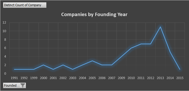
Next screenshot shows company distribution by Specialty. You can see the most common specialties for companies who specialize in PowerPivot (e.g. Business Intelligence, SQL Server and Excel).
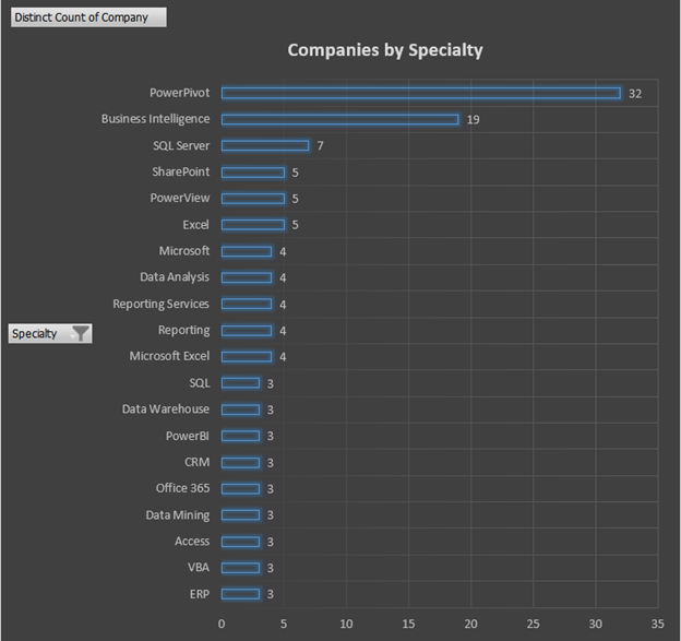
I am sure that by now, we got your attention 🙂
Before we start
Power Query doesn’t provide a dedicated LinkedIn connector (like Facebook, Salesforce, and Microsoft Dynamics CRM). As a result, the main challenge we will face is to authenticate to LinkedIn via external tool, get an access token to use its API, and then start using Power Query’s generic web service import capabilities (Power Query –> From Web).
LinkedIn background
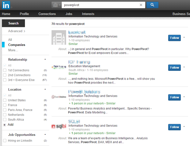
LinkedIn website provides easy user interface to search for companies by different criteria or certain keywords (see screenshot), but you cannot export the entire dataset to gain insights from the entire data.
For developers (or data enthusiasts like us) LinkedIn provides REST APIs that can be used for our purpose. If you are interested to learn more on the APIs, you can start here.
In this tutorial I used the company-search API call. For more information on that call go here.
Signing-in to LinkedIn (OAuth 2.0)
To use LinkedIn APIs, we will first need to obtain an access token from LinkedIn following a successful signing-in. The token is needed for all the API calls we will make. To learn more on LinkedIn OAuth 2.0 authentication go here.
LinkedIn provides an easy way for developers to test their Apps and learn APIs through REST console: https://apigee.com/console/linkedin
We will use this console to obtain the required access token, and use it with Power Query à From Web to extract the data we need.
This post is meant for learning purposes. Before you start building your solution, please follow the API Terms of Use here. Depending on the solution and the used API calls, you may need to register to LinkedIn Developer Program.
Ready to go? Let’s start.
Obtaining the access token
1. Go to the LinkedIn REST Console here.
2. On the Authentication dropdown menu select OAuth 2.

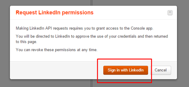
3. The Request LinkedIn permissions dialog will appear. Click Sign in with LinkedIn and follow the sign-in/permission process.
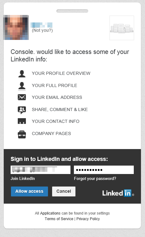
4. After you allow access to Apigee console, you will be back to the Console. On the left pane click Retrieve basic profile data, and click Send.
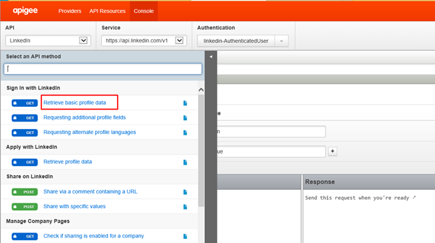
5. You will notice that the Request pane contains your access token (See selected blue area in the screenshot below). From the Request pane copy the access token to a notepad – This is the gibberish text that starts after “oauth2_access_token=” and is ends at “&format=json”
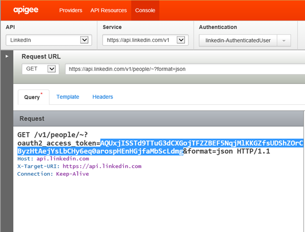
6. Congratulations you just obtained your LinkedIn access token. You will use this token later in Step 17. Note: This token can be used to retrieve personal information from your LinkedIn profile. Please don’t share it with others. In this tutorial, we will show you how you can use the access token, and share the workbook while the token never leaves your computer.
Building the query
7. Create a new workbook, go to Power Query ribbon and click From Web (If you are using Office 2016 Preview, click Data –> New Query –> From Other Sources –> From Web).
8. Copy the following URL to your notepad, and replace your access token from step 5 with the highlighted text:
https://api.linkedin.com/v1/company-search:(companies:(id,name,description,founded-year,employee-count-range,specialties,industries,locations:(address:(country-code,city))))?oauth2_access_token=paste the access token here&keywords=powerpivot&count=100&start=0&sort=relevance
9. Paste the URL and access token to the URL box of From Web dialog, and click OK
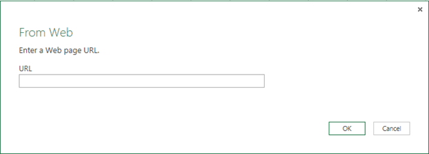
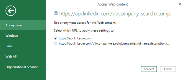
10. In Access Web content dialog, select Anonymous and click Connect
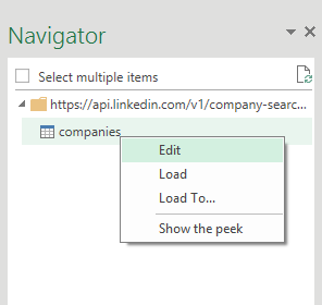
11. In the Navigator pane select companies and click Edit
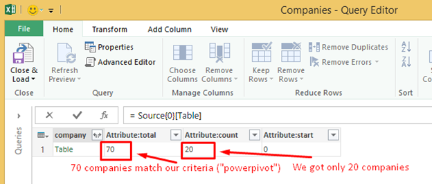
12. The Query Editor will open. You will see that Power Query extracted the table below, which contains 20 out of 70 companies that match our search criteria (Later we will show you how to get all the 70 companies using a function query, but one step at a time).
Removing access token from workbook
13. Before we continue to get the desired data from LinkedIn, let’s tune the M expression to ensure that the access token will not be stored in the workbook, and also to improve our query expression for future reuse.
In the Query Editor click View –> Advanced Editor
(Before you proceed, ensure that your access token is saved. We will delete it in a second from the M expression, but will need it soon one last time).
14. In the Advanced Editor dialog change the line that starts with “Source=” according to this table:
Before
Source = Xml.Tables(Web.Contents(“https://api.linkedin.com/v1/company-search:(companies:(id,name,description,founded-year,employee-count-range,specialties,industries,locations:(address:(country-code,city))))?oauth2_access_token=[access token]&keywords=powerpivot&count=100&start=0&sort=relevance“)),
After
apiURL = “https://api.linkedin.com/v1/company-search:(companies:(id,name,description,founded-year,employee-count-range,specialties,industries,locations:(address:(country-code,city))))“,Source = Xml.Tables(Web.Contents(apiURL, [ApiKeyName=”oauth2_access_token“, Query=[keywords=”powerpivot”, count=”20″, sort=”relevance”, start=”0″]])),
Let’s explain what we have done here:
· We created a text field called apiURL for the URL which is served for the Linkedin API Call, without its parameters.
· We moved all the URL’s parameters to a Query record.
· We removed the access token and declared that the field oauth2_access_token is the key that will be used as part of the Web API authentication.
15. Click Done in the Advanced Editor.
16. In the Query Editor click Edit Credentials (If you don’t see a yellow message bar with Edit Credentials button, click Home –> Refresh & Preview).
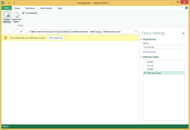
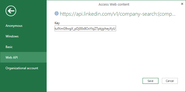
17. In the dialog Web Access content select Web API, paste the access token (which was obtained in step 6) in the Key textbox and click Save.
Interested in Learning How to Do this Kind of Thing?

Our New Online Power Query Course just launched this year. You’ll learn Power Query from the best in the business, two Excel MVPs Ken Puls and Miguel Escobar. We’ve included 7 Hours of Self-Paced Video over 31 Courses, with lots of example files, and a Digital Badge powered by Acclaim.
CLICK HERE to claim your spot.
We are now back in the query editor with an improved M expression that doesn’t reveal the access token. This change will allow us to share the workbook with others. New users who open the workbook will be able to edit the credentials with their token (after they obtain the token from LinkedIn API console as we did).
Let’s begin the transformation
18. Click the Expand button in the column header “company”, and click OK.
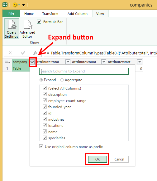
The Expand window gives us hint on the type of data we are going to get soon:
· Company name
· Description
· Employee-count-range (We will get the company size out of this field)
· Industries
· Locations (We will get the country codes and cities from this field)
· Specialties (This can be promising. We will be able to correlate between different specialties).
· Founded Year (Is PowerPivot adopted by old and mature consulting companies, or by younger ones?)
Figuring out the company size
19. Click the Expand button on the column header “company.employee-count-range”. Check the field “name”, check Use original column name as prefix and click OK.
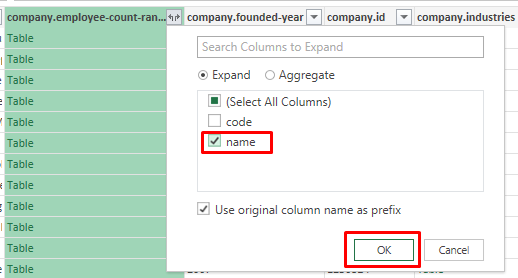
20. Rename column “company.employee-count-range” to “Size” (To rename the header, double click the header text and change the text).
You will notice that the column Size has a mixture of textual values. Some of those are ranges such as “2-10” or “11-50”, but there is also the value “myself only”. In the next steps we will transform this column into a column that shows the upper bound of each range (1,10,50, etc.)

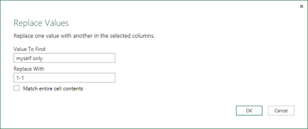
21. Right click the header “Size” and click Replace Values…
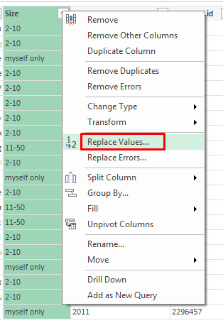
22. In the Replace Values dialog, write “myself only” in the Values To Find textbox, and “1-1” in Replace With textbox. Click OK.
23. Right click the header “Size” and click Split Column –> By Delimiter…
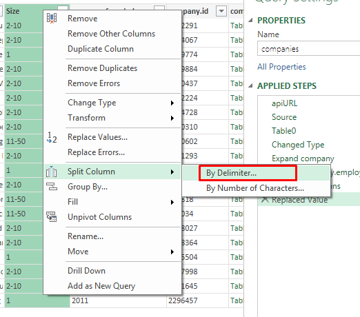
24. In the Split a column by delimiter dialog select –Custom—in the first drop down, type “–“ in the textbox, and click OK.

25. We now have two new columns instead of Size: “Size.1” for the lower bound and “Size.2” for the upper bound. As we are interested in the upper bound for the company size, let’s delete “Size.1” and rename “Size.2” to “Size”.
26. Delete the last 3 columns: “Attribute:total”, “Attribute:count” and “Attribute:start”.
27. Renaming the following columns:
a. company.description –> Description
b. company.founded-year –> Founded
c. company.id –> Id
d. company.name –> Company
Where is my Geo-location? (where should I start my next PowerPivot consulting branch?)
28. Click the Expand button on the column header “company.locations”. Check the field “location”, uncheck Use original column name as prefix and click OK.

29. Click the Expand button on the column header “location”. Check the field “address”, uncheck Use original column name as prefix and click OK.
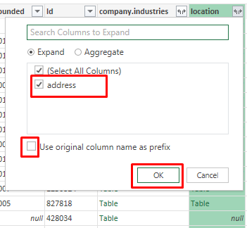
30. Click the Expand button on the column header “address”. Check the fields “city” and “country-code”, uncheck Use original column name as prefix and click OK.
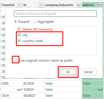
We now have the geo-location data that is needed to build cool visualizations with Power Map.
Industrious step ahead
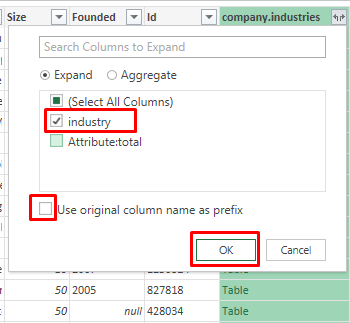
31. Click the Expand button on the column header “company.industries”. Check the field “industry”, uncheck Use original column name as prefix and click OK.
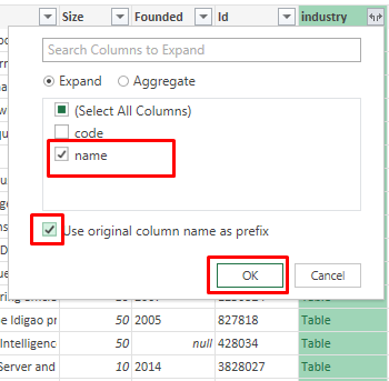
32. Click the Expand button on the column header “industry”. Check the field “name”, check Use original column name as prefix and click OK.
33. Rename the column “industry.name” to “Industry”.
Special Specialty (Part 1)
34. Click the Expand button on the column header “company.specialties”. Check the field “specialty”, uncheck Use original column name as prefix and click OK.

35. Click the Expand button on the column header “specialty”. Check the field “Element:text”, uncheck Use original column name as prefix and click OK.

36. Rename column “Element:Text” to “Specialty”.
Special Specialty (Part 2) – How to expand a column with mixed types of tables and text
Let’s test our query, and change the M expression to call for the next 20 “powerpivot” companies (by changing the highlighted text from “0” to “20”:
Source = Xml.Tables(Web.Contents(apiURL, [ApiKeyName=”oauth2_access_token”,
Query=[keywords=”powerpivot”, count=”20″, sort=”relevance”, start=”20″]])),
The Query Editor will now show three types of values under the column “specialty”: Table, null and text. Our new challenge is that the expanding we performed on the previous step will yield an error as Power Query cannot expand text. Let’s see how this can be fixed using custom columns and simple if-then-else statements.

37. Delete the last two steps (Expanding “specialty”, and renaming “Element:Text” to Specialty).
38. We will now add two custom columns. Into the first column we will copy all the tables from column “specialty”, so we will be able to expand it. Into the second column we will copy all the text values from column “specialty”. Then we will have two columns that can be merged.
39. Click Add Column –> Add Custom Column.
40. In Custom column formula textbox write:
= if ([specialty] is table) then [specialty] else null

41. Click OK
42. Now we will create the second custom column. Click Add Column –> Add Custom Column.
43. In Custom column formula textbox write:
= if ([specialty] is table) then null else [specialty]
44. Click OK
We now have two new columns: Custom with all the tables, and Custom.1 with the text values.
45. Delete the original column “specialty”.
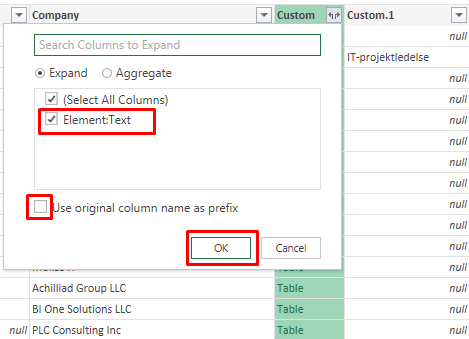
46. Click the Expand button on the column header “Custom”. Check the field “Element:text”, uncheck Use original column name as prefix and click OK.
47. Select the two columns “Element:Text” and “Custom.1”, right click and select Merge Columns

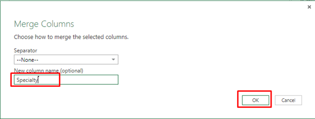
48. In the Merge Columns dialog select “–None–“ as the separator, and “Specialty” as New Column Name, and click OK.
Scaling it up – From 20 companies to all
As LinkedIn limits the results to 20 companies per API call, you will now see how to use Power Query to fetch all companies (Note: Even if we explicitly try to fetch more companies by using the count parameter, we can only get 20 companies).
As we know that there are 70 PowerPivot companies, we will turn the query into a function query and will call it 4 times with the relevant offset (ranging from 0 to 60). In the last section we will also show you the M expression which can dynamically decide how many calls are needed, so you will not need to know in advance how many API calls to use.
49. To create a function query, we will start by renaming our query from “companies” to “getCompanies”
Well, this is not enough to turn the query into a function query, but it’s a start 😉
50. Now let’s edit the first few lines of the query expression according to the table below (Edit the query, and click View –> Advanced Editor).
Before
letapiURL = “https://api.linkedin.com/v1/company-search:(companies:(id,name,description,founded-year,employee-count-range,specialties,industries,locations:(address:(country-code,city))))”,Source = Xml.Tables(Web.Contents(apiURL, [ApiKeyName=”oauth2_access_token”, Query=[keywords=”powerpivot”, sort=”relevance”, start=20, count=”20″]])),
After
(offset as text, inputKeywords as text) =>letapiURL = “https://api.linkedin.com/v1/company-search:(companies:(id,name,description,founded-year,employee-count-range,specialties,industries,locations:(address:(country-code,city))))”,
Source = Xml.Tables(Web.Contents(apiURL, [ApiKeyName=”oauth2_access_token”, Query=[keywords=inputKeywords, sort=”relevance”, start=offset, count=”20″]])),
51. After you made the changes in the Advanced Editor click Done.
You will see that the query was turned into a function query. It’s time to save this query.
Click Home –> Close & Load.
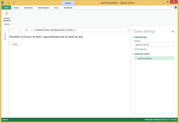
52. Create a blank query by clicking Power Query –> From Other Sources –> Blank Query (If you use Excel 2016 Preview click Data –> New Query –> From Other Sources –> Blank Query).
53. In the formula bar write:
= {0..3}
Type Enter
54. Type Enter and click To Table and click OK in the To Table dialog.
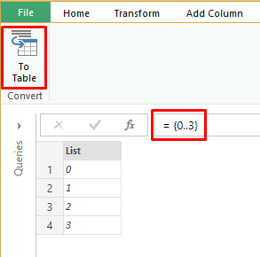
55. Add a new column that multiply the first column by 20. This can be done by clicking Add Column –> Standard –> Multiply
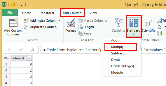
56. Type the number 20 in the Multiply dialog and click OK.
57. Delete Column1 and rename “Inserted Multiplication” column to “Offset”.
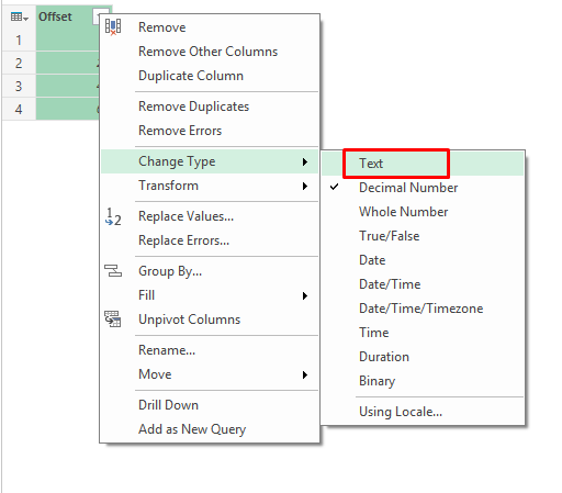
58. Change “Offset” type to Text by selecting the column “Offset” right click and click Change Type –> Text
59. Click Add Column –> Add Custom Column and in the Custom column formula textbox write
=getCompanies([Offset],”powerpivot”)
Click OK in the Custom Column Dialog.

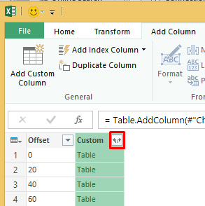
60. Expand the column “Custom” by clicking the Expand button (marked below).
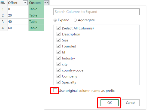
61. Ensure all columns are selected. Uncheck Use original column name as prefix, and click OK.
62. Delete “Offset” column
63. Click Home –> Close and Load to… and select Add this data to Data Model
64. Let’s name this query “LoadAllCompanies”
Scaling it up even further
Previously we used a predefined list {0..3} to iterate over the 70 PowerPivot companies. We also used the keyword “powerpivot” inside the Power query expression. At this final section, we will build parameterized query the loads the search keywords from the workbook, and dynamically iterate LinkedIn API to extract all the search results (without knowing in advance the number of companies that the search will yield). To know the number of companies in advance we will build a new query that gets reads the attribute “Attribute:Total” from LinkedIn (We saw it above in step 13).
65. We will create a new function query (using Blank Query)
(inputKeywords as text, max as number) as number =>
let
apiURL = “https://api.linkedin.com/v1/company-search:(companies:(id,name,description,founded-year,employee-count-range,specialties,industries,locations:(address:(country-code,city))))”,
Source = Xml.Tables(Web.Contents(apiURL, [ApiKeyName=”oauth2_access_token”, Query=[keywords=inputKeywords, sort=”relevance”, start=”0″, count=”1“]])),
Table0 = Source{0}[Table],
#”Changed Type” = Table.TransformColumnTypes(Table0,{{“Attribute:total”, Int64.Type}, {“Attribute:count”, Int64.Type}, {“Attribute:start”, Int64.Type}}),
#”Removed Columns” = Table.RemoveColumns(#”Changed Type”,{“company”, “Attribute:count”, “Attribute:start”}),
#”Renamed Columns” = Table.RenameColumns(#”Removed Columns”,{{“Attribute:total”, “Total”}}),
companyCount = #”Renamed Columns”[Total]{0},
returnNum = if (companyCount > max) then max else companyCount
in
returnNum
The input parameter “max” will be used to limit the number of Linkedin calls we will conduct.
66. Save the new query and rename it “getCompaniesCount”.
67. We will also adjust “LoadAllCompanies” query to get the keywords from a table in the workbook. The keywords will be located in a simple Table named “Keywords” with a single column and a header named “Keywords”. The single cell will include our keywords (As shown in the screenshot below).

68. We will now edit “LoadAllCompanies” with the advanced editor and change the expression to the following one (The changes are highlighted):
let
keywords = Excel.CurrentWorkbook(){[Name=”Keywords”]}[Content][Keywords]{0},
lastNumberInList = Number.RoundUp(getCompaniesCount(keywords, 500) / 20),
Source = List.Numbers(0, lastNumberInList),
#”Table from List1″ = Table.FromList(Source, Splitter.SplitByNothing(), null, null, ExtraValues.Error),
#”Inserted Multiplication” = Table.AddColumn(#”Table from List1″, “Inserted Multiplication”, each List.Product({[Column1], 20}), type number),
#”Removed Columns” = Table.RemoveColumns(#”Inserted Multiplication”,{“Column1”}),
#”Renamed Columns” = Table.RenameColumns(#”Removed Columns”,{{“Inserted Multiplication”, “Offset”}}),
#”Changed Type” = Table.TransformColumnTypes(#”Renamed Columns”,{{“Offset”, type text}}),
#”Added Custom” = Table.AddColumn(#”Changed Type”, “Custom”, each getCompanies([Offset], keywords)),
#”Expand Custom” = Table.ExpandTableColumn(#”Added Custom”, “Custom”, {“Description”, “Size”, “Founded”, “Id”, “Industry”, “city”, “country-code”, “Company”, “Specialty”}, {“Description”, “Size”, “Founded”, “Id”, “Industry”, “city”, “country-code”, “Company”, “Specialty”}),
#”Removed Columns1″ = Table.RemoveColumns(#”Expand Custom”,{“Offset”})
in
#”Removed Columns1″
The section in yellow imports the keywords from our table. The section in green invokes “getCompaniesCount” to know the total number of companies that LinkedIn search should yield, it then calculates the number of API calls that are needed by using Number.RoundUp divided by 20 (the number of companies we get per call).
69. Save the modified query, and refresh the query.
70. Rejoice!
Finish Line!
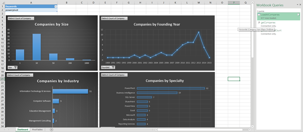
That’s it. We have just walked through seventy steps to build the ultimate queries for your competitive analysis dashboard. You are encouraged to take the workbook here to see the Dashboard we have created with these queries.
Note: Since we removed the access token from the workbook, if you share your competitive analysis dashboard, please share the instructions on how to get the token from LinkedIn Console (steps 1 to 6), and use the token in the Key textbox (as shown in step 17).

Get in touch with a P3 team member