A long time ago I did a post on using slicer selections in Excel formulas. That technique only worked when you select single values on slicers, though – any more than one and the dreaded “(Multiple items)” foils your well-laid plans.
How to handle that multi-select case became a very common question – in email and posted as comments.
Awhile back I responded privately to one of those requests but haven’t had time to post the solution. So here goes.
The Solution, Summarized
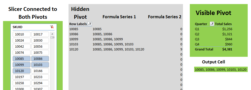
First, here’s a picture of the solution I came up with. For fun, see if you can figure out what I’m doing just by looking at it:

Everything in green is visible to the final report consumer (or at least, you can choose to make it so). Everything in grey is stuff you likely hide – either by hiding columns or by placing on a hidden sheet. The SKUID field is on the slicer (that is hooked to both pivots) and is also on the row axis of the hidden pivot, but is not included on the visible pivot.
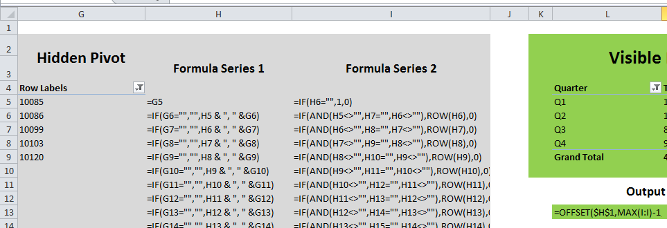
Here’s the same spreadsheet, but zoomed in and with formulas visible:

I went ahead and uploaded this workbook so you can take a look in a hands-on manner.
CLICK HERE TO DOWNLOAD THE WORKBOOK
Note that this was a PowerPivot workbook originally but I think I nuked all the data out of it, so you won’t be able to manipulate the pivots. No worries though – the formulas here are 100% of the technique and should work with any pivot.
I’m pretty sure I could simplify this a little bit if I tried, but probably not by much. I eagerly await everyone’s constructive input
Update, November 2012
I’ve since posted yet another way to do this that is probably the simplest I’ve personally used to date, and it handles multi select quite well too:
Get in touch with a P3 team member