Break your DAX Problem into Manageable Parts

One of the concepts I discuss in my new book Learn to Write DAX, is that you should break your DAX problems into manageable pieces so that you can solve the problem one step at a time.  Most of us do this intuitively in regular Excel, and it should be no different for Power Pivot and DAX.  The trick is to create test measures that are used simply to solve one part of the problem.  Once you have worked out each piece of the problem independently, then you can use the learnings from the test measures to create the final working solution.  This blog post is more about that process of breaking the problem into pieces rather than the specific solution proposed.  This solution may not be the best solution, certainly not the only solution, and probably not the most performant solution.  I am thinking there may be a DAX Query solution using GENERATE and maybe CALCULATETABLE (after watching an Alberto Ferrari video last night), but in this post I just want to focus on how to break the problem into manageable pieces so you can actually get a working solution.  Once you have a working solution, you may then want to find a better solution if needed (the topic for a future blog post maybe).

A Tricky Little Golf Problem

I was helping Michael (a regular) at https://powerpivotforum.com.au with a tricky little golf problem.  Actually, truth be known, all of Michael’s golf problems are tricky .  He uses Power Pivot for Excel to administer his golf handicapping at his local golf club because Power Pivot can handle many millions of rows of data.  Without Power Pivot, he would need to move to Access or some other database tool.

First the solution

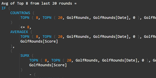
I want to start by providing an answer.  The point I want to make here is that this is a super complex formula.  But YOU and everyone else reading this blog CAN DO THIS if you follow the principles I describe here.

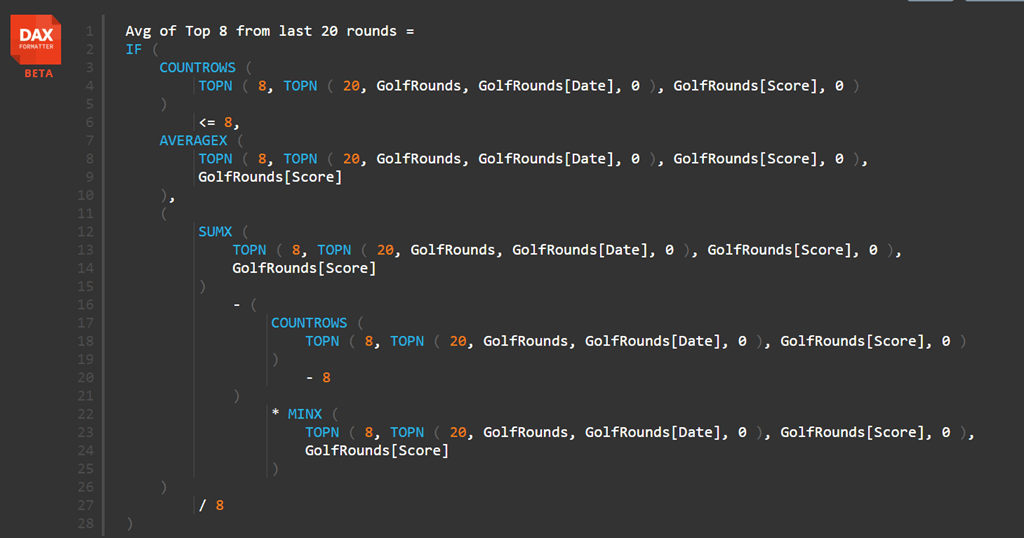
I promise you I didn’t (and couldn’t) write this formula from scratch.  But I can (and did) write this formula using the method I am about to describe to you (and it works by the way ).

Edit:28th Nov.  Note I mentioned above this was “an answer” and I was sure it wasn’t the best answer.  There is a better answer provided below from a couple of readers who posted comments.  But read on.  This post is about using test measures to help solve DAX problems.

Average of best 8 scores from last 20 rounds

So the requirement is to find the average of the best 8 scores from the last 20 rounds of golf for each player.  So if you think about that problem, there are quite a few layers to it – perfect for a blog on how to break a problem into pieces so you can solve it in DAX.

The DAX Problem Solving Process

In my experience, the best way to solve a problem in Power Pivot with DAX is to follow the following process.

1. Write down (or at least think about) the problem in English (or any other language of choice).
2. While still in language form, break the problem into logical manageable pieces.
3. Create a DAX formula to solve each piece of the problem on its own using one or more test measures.
4. Combine the learnings from each piece of the puzzle from step 3 to create your final working solution.

This will all make more sense with a working example, so let’s do that.

1. Write down the problem in English

So here is my English language definition of this problem.

Find the average of the best 8 scores from the last 20 rounds of golf for each player.

2. Break the Problem into Manageable Pieces in English

1. Create a table that contains just the last 20 rounds of golf for each player – based on the latest dates.  (may be less than 20 rounds for some players if they have never played 20 rounds).
2. From this table, keep only the best 8 rounds – based on the best score (stableford – higher score is better).
3. From this second (now further reduced) table, work out the average score

All of a sudden the problem seems manageable now that we have chopped the elephant up into pieces.

3. Solve Each Piece of the Puzzle in DAX with Test Measures

Here is what the sample data looks like

Note there is:

• an ID column (ID of the player)
• a Date column for the date of the round
• a Score column (stableford – larger is better).

This is test data stored as a linked table in the sheet (not ideal in real life but fine for testing).

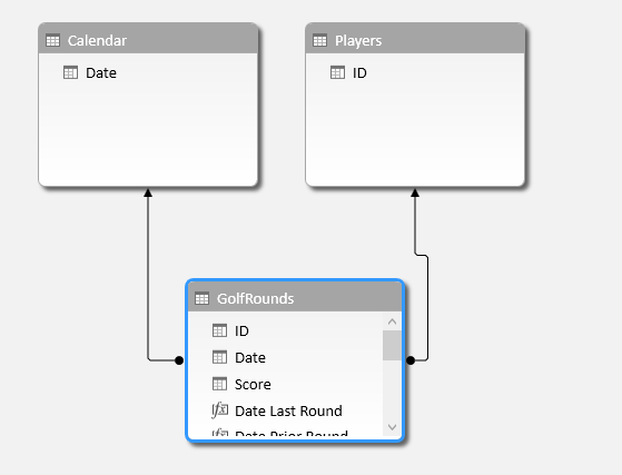
Create Lookup Tables

The next thing I did was create 2 lookup tables using Power Query.  It is good practice to do this as Power Pivot is optimised to operate over this data model shape.  To do this, I did the following:

• I created a link to the sample golf round data in Power Query – create connection only.
• Create a new query pointing to query 1 and called it Calendar
  • I kept only the date column and removed all other columns.
  • I then removed duplicates and loaded the calendar to the data model
• Create another new query pointing to query 1 and called it Players.
  • I kept only the Player ID column, removed duplicates and loaded it to the data model.

Then I joined all the tables together as shown below.

Only now is it time to write some DAX.

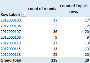
The first measure I wrote is [Count of Rounds].  It is not required for this analysis, but I think it is always good to get some early runs on the board (sorry, that is a Cricket Idiom).

As you can see in the pivot above, I have Players[ID] on Rows, and my new measure [Count of Rounds] in values.  This is really good test data as I have some players with more than 20 rounds, and some with less than 20 rounds, and some with a lot less than 20 rounds.  As I often say in these posts, it is essential to have good test data if you want to get it right the first time.

Task 1 – create a table of last 20 rounds

Remember the English description from above?  Create a list that contains just the last 20 rounds of golf for each player – based on the latest dates.  (may be less than 20 rounds for some players if they have never played 20 rounds).

When I write a DAX measure I can’t actually return a table into the pivot.  I could use DAX Studio to create a table, and actually that would be a good approach for harder problems.  But in this case all I really need to do is first create the table and then wrap the table in a COUNTROWS() formula so that I can get some visual confirmation that my formula is working.

The formula that returns a table of the last 20 rounds for the current player is as follows:

Table of last 20 rounds =TOPN(20,GolfRounds,GolfRounds[Date],0)

A quick Google for the syntax of TOPN tells me that the last parameter (zero above) means “sort descending”, so 0 means latest rounds at the top.

But I can’t put this table into my pivot, so instead I created the following test measure

Count of Top 20 Rounds = countrows(TOPN(20,GolfRounds,GolfRounds[Date],0))

When I add this measure to my pivot, I get good visual confirmation that I am on the right track. Note how below the column on the right is never more than 20, but when the count of rounds is less than 20, then the count of top 20 rows is also less than 20 – perfect.

Task 2 – keep only the best 8 rounds

Now that I have a formula that I know returns the latest 20 rounds, I can pass this table I just created into another formula.  I am not talking about the test measure [Count of Top 20 Rounds] here, I am talking about the table INSIDE the [Count of Top 20 Rounds]

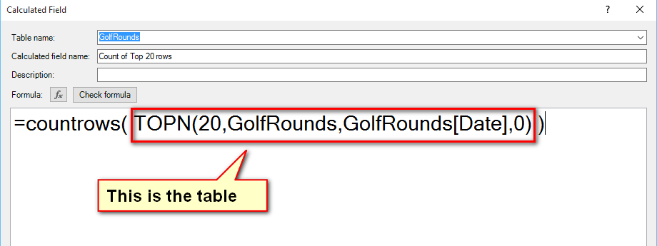
So now I write another test measure that generates a table of the Top 8 best rounds using the above table in the red box as the starting point.  I need to wrap this new table inside a COUNTROWS() again for the same reason as above.  Note the original table from above is highlighted in bold below.

Count of Top 8 Rounds =countrows (
TOPN ( 8, TOPN ( 20, GolfRounds, GolfRounds[Date], 0 ), GolfRounds[Score], 0 )
)

When I add this test measure to the pivot, I get the following.

Houston, we have a problem!

Note how the last player has 10 rounds in the top 8.  How is this possible?  Time to go back and check the source of the test data for this player.  Good thing I have realistic test data, ‘else i would have missed this problem.

When I looked at the raw data, the problem became obvious.  Note below how the 8th round has a score of 19, but this is the same score for the 9th and 10th round too.  So basically there is a tie for 8th best round, an hence round 9 and 10 are included in the table too.

This is bad for me.  I did some more Googling and couldn’t find a way to add a DENSE flag – to ignore all rounds greater than 8 when a tie occurs – not for Excel 2013 anyway. There seems to be a solution for Excel 2016 however.  Maybe someone else knows better.  Anyway, I came up with a creative solution, once again by thinking about the problem in plain English first, then breaking the problem into a DAX problem.

If it were not for this above problem, I could just use a simple AVERAGEX as follows:

Average of Top 8 Rounds = averagex (
TOPN ( 8, TOPN ( 20, GolfRounds, GolfRounds[Date], 0 ), GolfRounds[Score], 0 )
,GolfRounds[Score])

But I have to manage the ties.

Breaking the problem into pieces, I first worked out which players had a problem – those players that have [Count Rows of Top 8] > 8.  In other words, any player that had more than 8 “top 8” rounds, had a tie for 8th.    So I then created a measure to check what the minimum score was for the Top 8 Rounds as follows.

Min of Top 8 = minx (
TOPN ( 8, TOPN ( 20, GolfRounds, GolfRounds[Date], 0 ), GolfRounds[Score], 0 )
,GolfRounds[Score])

The next step was to add up all the scores for all “Top 8 Rounds”.

Sum of Top 8 =

Sumx (
TOPN ( 8, TOPN ( 20, GolfRounds, GolfRounds[Date], 0 ), GolfRounds[Score], 0 )
,GolfRounds[Score])

Note the repetition of the same input table in the 3 formulas above (in bold).  This input table is the one i developed earlier with my test measures.

Finally, using all these interim measures, I can calculate the average of the Top 8 as follows.

Complex Average of Top 8 = if([Count of top 8 rows] <=8,[Average of Top 8],([Sum of Top 8]-([Count of top 8 rows]-8) * [Min of Top 8])/8)

In English this formula reads as follows:

If there are 8 or less rounds in the top 8, then just use the simple top 8 formula.  But in the case where there are more than 8 rounds in the top 8 (ie there are ties), then first add up all the scores in the top 8, and then subtract the smallest score once for each tie greater than 8.  So if there are 9 scores, then subtract the minimum score once.  If there are 10 scores, then subtract the minimum score twice, etc.  After that you will have the aggregate of the top 8 scores, and you can then divide by 8.  Simple!!

OK, but here is the point.  No one ever could write the following formula from scratch, starting at the top line and working down the formula – this is simply not possible and not the way it is done.

But this formula works – check it out in the sample workbook if you like.

The Moral of the Story

The whole point of this blog post is to describe the process of problem solving in DAX.  The final DAX formulas always look complex.  When you read a formula like the final one I show above, it is natural to think “how the hell did you write that formula?”.  But the point is that NO ONE writes these from scratch – not even in Italy.  Everyone that writes complex DAX formula breaks the problem into pieces and then solves one piece of the problem at a time.  Once you have done that, you can conquer the world.

If you want to learn about interim formulas and other tips to writing DAX. then check out my new book here.

Edit: A Better Answer (28th Nov)

As you can read in the comments below, Jes provided an insightful solution to solving the tie problem using RAND().  In fact Jes said that he only discovered the solution when he put the problem on paper – and then it jumped out at him.  This is one of the key points of this post – first think about the problem without considering the DAX language, then convert the solution into DAX. Here is that solution.

Note below the syntax of TOPN allows for multiple sort columns (order by expression 2 etc).

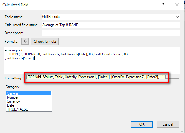
The idea that Jes came up with is to use the RAND() function as the second sort order column.  By doing this, it makes every row unique (assuming the 1 in a million chance that you wont get a tie with the random number) and once each row is unique, there are no longer any ties – brilliant!

Take a look at the sample data with this new RAND column added in the image below.  In reality this column doesn’t exist in the table, but instead it is added on the fly just during the TOP8 calculation.

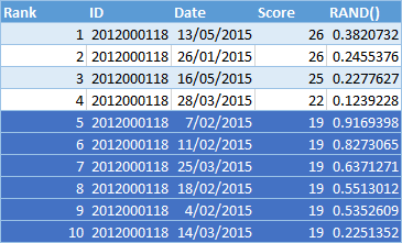
Notice the ties in rows 5 through to 10 (all have a score of 19).  But once you add the RAND() column, each row is now unique and hence there is no longer a tie.  With this new column added, the TOP8 function works.

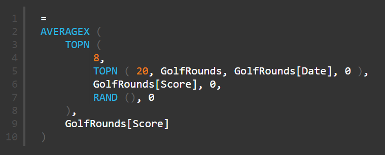
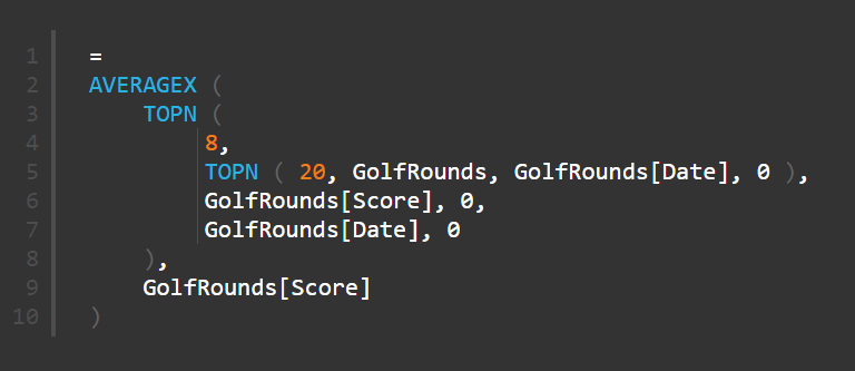
Once I understood what Jes had done here, I then realised that I could use the date column as a method of breaking the ties too (as long as there was not 2 games on the same day by the same player with the same score (unlikely in this case). So hence this formula also works.

Some things to take away

• A problem shared is a problem halved. If you have a problem you are stuck on, or you want to improve on, then consider posting it at https://powerpivotforum.com.au and ask others to help. Everyone benefits when you do this. You benefit, the person helping benefits, and others reading the problem benefit.
• As I mention in my book, you CAN incrementally learn Power Pivot and DAX, but only of a solid base of understanding. Once you have that solid base, you can incrementally learn – just like many of use have learnt something from a post like this.
• It doesn’t matter whether you end up with the complex DAX I first created, or a better solution like the one discovered by Jes.  You will definitely find it easier to solve the problem by breaking it into logical pieces and solve each piece of the problem with a test measure first.