Arriving Here from a Search Engine or via Excel Help?
This article below by Dick Moffat, as well as the one by Dany Hoter, is an excellent, detailed example of how to use cube functions with *any* OLAP data source, and NOT just PowerPivot. Cube functions work the same with PowerPivot as they do with other OLAP sources like Analysis Services.
I highly recommend reading both for examples and ideas.
But if you want to use cube functions with just plain tables of regular data, you can do that with Excel 2010! Just download PowerPivot (free addin from MS), copy/paste or link your tables of Excel data into PowerPivot sheet tabs, and you are off and running. The New Visitor page has information on how to get started, including download links.
And now, on to Dick’s excellent article…
Using Excel Cube Functions with PowerPivot
By Dick Moffat
Personal Logic Associates Inc.
Today I am going to give you a quick and dirty example of what I think is one of the key features of PowerPivot that will give it a much broader initial and on-going impact for experienced power spreadsheet developers.
This is where existing spreadsheets can get the value-add of having PowerPivot data available to them in a way that is not only understandable for the traditional spreadsheet junkie (as opposed to the typical BI one) but that also that will add major value while integrating into existing models.
Excel CUBE Functions
A few weeks ago my friend Dany Hoter wrote a piece here about the use of the CUBE functions in Excel with PowerPivot data. Dany’s article was a great intro to the capability of this unsung capability of Excel available since Excel XP. I am going to go deeper into this issue here.
The Cube functions require access to an Analysis Services On-Line Analytical Process cube (OLAP) which has to be provided to the user from SQL Server’s Analysis Services application.
While there are companies around the world that are capable of taking advantage of this capability, this is by no means a large percentage of overall Excel users and from my experience it is generally an unknown and untried feature.
In Excel 2007 (and now 2010) the CUBE functions became native to Excel (as opposed to available through an Add-In) and were integrated with the new “Connection” object within the program. Once again though, if one wanted to use an OLAP Cube in a Connection it required availability of an Analysis Services Cube of data.
But in Excel 2010, thanks to PowerPivot, users can now create their own “Cubes” inside PowerPivot and they automatically present themselves as an available Connection inside the Excel parent file. This is a big thing and I hope to show you another reason why.
A Cube Automatically?
I’m sure I don’t have to explain here how one creates a PowerPivot data source consisting of multiple Relational data sources. But one fact that may not be obvious is that the data set that is created by these PowerPivot objects, and by their relationships, is in fact a “Virtual” Cube in itself. In the purest sense it is a ROLAP Cube – created at run-time from Relational data.
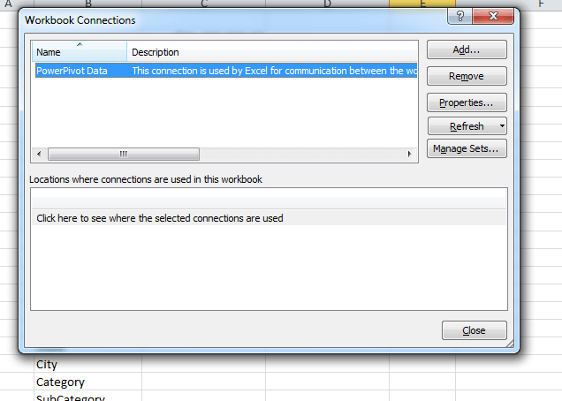
This default “Virtual” Cube is named “PowerPivot Data” and is exposed when you click the Connections Button on the Data Tab:

This is inherently an OLAP Cube conceptually and so is an acceptable source for Excel’s native CUBE Functions.
So what does this “Cube” Do For me?
OLAP “Cubes” were designed for two major reasons:
- To allow analysis of data in a hierarchical fashion. In the business world that usually means Financial or Sales or other data organized by the hierarchy of business units (Region/Country/Zone/State/County/City) or by dates (Year/Quarter/Month/Week/Day) or by Product lines (Product Category/Product/SKU), where a number or numbers (i.e. Account balances or sales quantities or values) are stored at the lowest level of detail (i.e. by Day or by SKU) and the total value or quantity can then be “Rolled Up” along any Hierarchy or Dimension and across dimensions. So for example you want to see total sales for March 2010 of a particular Product and its SKUS in a particular Country…. Then you want to be able to “Drill up” or Drill Down” on any value in any dimension down to the lowest level or up to the highest easily and automatically. This is where a Pivot Table attached to one of these Cubes is a natural presentation and analysis mechanism.
- To take disparate data sources and aggregate them automatically using the hierarchies in 1 above. In the original implementations of OLAP Cubes the hardware available had limited RAM and slow processors and so many OLAP Cubes had to be created over-night and written to disk in the classic De-Normalized format that allowed for relatively quick queries to be made against data that otherwise would simply not be possible in a Normalized format. But this is the 21st Century with incredibly cheap and sizable RAM memory on every PC and with processors so fast that it’s hard to believe. This is the work that PowerPivot is designed for – so it can reconstitute your OLAP “Virtual” Cube at run-time inside your Excel file itself (and with compression to boot).
So if you bring in your sales data (like in the example Bike data available with PowerPivot samples) and set it up in a PowerPivot “Connection” you can refer to that info from your spreadsheet layer using not just Pivot Tables, but also using the Cube functions. But the Cube functions give the traditional spreadsheet maker (and his/her boss) the flexibility to present this data in the classic free-form spreadsheet style as Income statements with analysis or to group them on the sheet in any way they want.
The Example
The data being used in this example is available in the “AW_CompanySales.accdb” database supplied as an example for use with PowerPivot. Keep in mind that there are many “Memo” field-types in this example database and it would be worth your while to change most of those fields to a Text format and add a few Indexes to improve the performance of the database when importing into PowerPivot.
This is an example of what the key tables look like when imported into PowerPivot :

When you create Relationships between these tables within PowerPivot, the result is a Virtual Cube with the ability to “Roll-Up” the core values (“Facts”) along any Dimension of the data, which actually are fields in the data sources of the table being used for Hierarchical relationships. So Product Categories in the “ProductCategory” table have children in the “ProductSubCategory” table, which have children in the “Product” table. This is the fundamental design of a “Snow-Flake” OLAP design (read about it!) and it should be fairly intuitive to anyone who knows the data sources and how they are related conceptually.
In my example, however, I have pulled together this same data into a single large De-Normalized PowerPivot table by creating an Access Query. The result is exactly as PowerPivot does virtually within its “PowerPivot Data” Connection and hopefully will help me explain this functionality better.
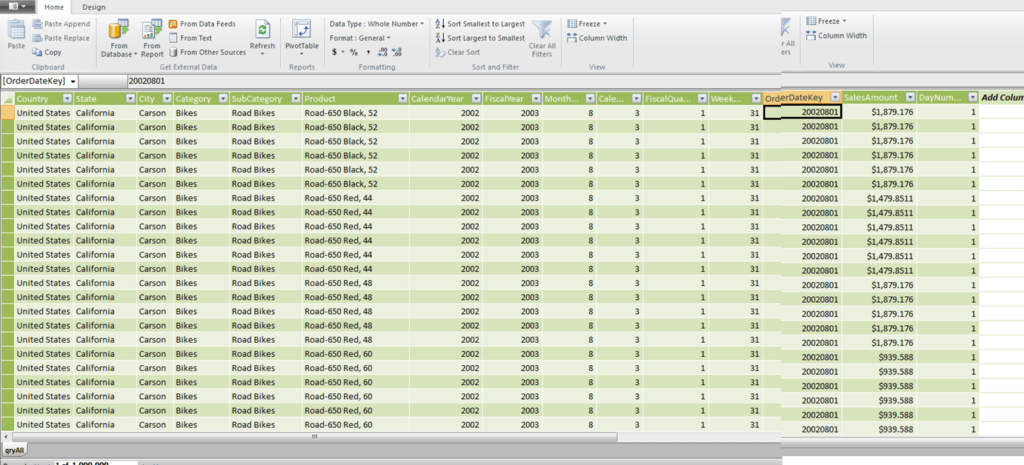
This is how that PowerPivot window looks (in an unfortunately stiched together image I’m afraid):

Do you notice how there are multiple instances of Country and State across records (?) This is in effect a result set from an Access query or SQL View or SQL Statement and is truly de-normalized. There will be certain scenarios where this might work to your advantage over bringing in individual tables and joining them inside PowerPivot, but that’s an issue for another day. There is little or no impact on file size for the two ways of importing the source data however. It is meant to help us see our data easier in this example.
Keep in mind that there are a million daily records in this data set and is a recipient of the exceptional compression algorithms of PowerPivot. It is also worth noting that the single table de-normalized version is 1/10th the size of the file with multiple tables (3 megabytes compared to 30 megabytes).
The “Measures”
Once you have the data in place within PowerPivot you have to take the next step and create the Measures you will be working with. Measures are the core of OLAP Cubes and are also the core of PowerPivot. Measures are the aggregations that you will be analyzing based on the data in columns you wish to SUM or COUNT or AVERAGE (or whatever of the standard Excel Mathematical and Statistical functions you want to use).
The most basic example of a Measure is ours called “[Sum of SalesAmount]’, where it simply sums the [SalesAmount] column at every conceivable level of the Virtual OLAP Cube inside Excel, created by PowerPivot. In this case [SalesAmount] is simply a basic data column provided directly from the data source, but there is no reason why you can’t use DAX to create new Calculated Fields of calculated data and then create “Measures” based on those fields.
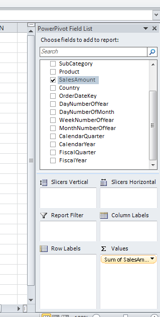
To create the aggregations you want in your spreadsheet you need to have created the “Measure” inside a Pivot Table in the Excel environment either within the “drag and drop interface or using the menus. I created our Measure using the Pivot Table interface like this:

I started to create a Pivot Table from inside my PowerPivot environment (or in the Excel environment from the PowerPivot Tab), and then I dropped the [SalesAmount] field from my Field List into the Values section below. By default the Pivot Table assigned this as a “SUM” function and it created the Measure [Sum of SalesAmount] automatically. It is now available to the Workbook, not only to any Pivot Tables you might create, but also to any CUBE functions that you might want to use.
This does NOT mean you have to have a Pivot Table in your Workbook, BUT you do have to have started the process in order to create the Measure or Measures you want to refer to in your CUBE functions. You can create the Measures from within the PowerPivot Pivot Table menu as well, but using the Excel Pivot Table GUI this way strikes me as more intuitive and equally capable. We can then rely on this Measure to aggregate the total “Sales Amount” at every level across any Dimension in our Virtual OLAP Cube.
The Spreadsheet:
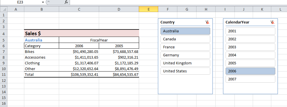
So here’s the spreadsheet I want to feed from PowerPivot:

The CUBEVALUE() Function
In order to drive right to the heart of this functionality I am going to use just one of Excel’s Cube functions, CUBEVALUE in this model (but will show one more function later as well in an enhanced version).
So we are looking for the Sum of the Sales Amount ([SumofSalesAmount]) of Bikes ([Category]) for Fiscal Years 2006 ([FiscalYear]) for Australia ([Country]). So this is the pseudo-code for this formula:
Sum the Sales Amount where Category = “Bikes” and Fiscal Year = 2006 and Country = “Australia”
Notice that the values are in the PowerPivot tables at the lowest level by Product, by City, by Date of the “Fact” Sales Amount. Each value is shown as a member of a Week and Fiscal and a Calendar Month and a Fiscal and a Calendar Year.
So when we ask for values from the Fiscal Year, the Category and the Country fields we are inherently asking for aggregated totals ate the intersection of those three fields. That is what you do when you look for values in an OLAP Cube.
This is the CUBEVALUE() function to get this value for “Bikes” in Australia for Fiscal 2006 :
=CUBEVALUE(“PowerPivot Data”,”[Sum of SalesAmount]”,”[Country].[Australia]”,”[Category].[Bikes]”,”[FiscalYear].[2006]”)
Which returns a total of $91,490,280.05.
Therefore to get the equivalent value for “Accessories” in Australia for 2005 the formula would be:
=CUBEVALUE(“PowerPivot Data”,”[Sum of SalesAmount]”,”[Country].[Australia]”,”[Category].[Accessories]”,”[FiscalYear].[2005]”)
And the result is $902,316.21.
If you have ever used a SUMIFS Function in Excel (or SUMIF or even IF functions) then this kind of formula is pretty straightforward IMHO.
The “Inherent” Connection
Notice that this function is a DIRECT reference to the “PowerPivot Data” Connection rather than referencing another cell that has a reference to the Connection? If you were connecting to an external data source you would likely want to make a single cell the one that links to the data source and then you would “borrow” that link for all subsequent references to the Cube. Otherwise you would have a HUGE performance hit.
But if the Connection is a “Virtual” Connection in PowerPivot inside the spreadsheet itself, then there is no such penalty. So you can refer to the “PowerPivot Data” inherent connection in every formula. That is much easier to understand and to audit as well.
Adding the Power of Excel to the Mix
As a loooong-time spreadsheet user I have developed a fondness for the “Naming” capability of Excel. By applying a “Name” to a cell or cells I can then refer to them everywhere in the Workbook without regards to the actual Sheer and Cell reference of the range. This makes things more auditable and just generally more readable.
In addition, I believe in the use of cell references for Variables in formulae rather than hard-codes words and values. To an experienced Spreadsheet developer this is simply “Best Practices”, but I still see many instances of “Hard-Coding” in Workbooks that make me cringe. If the value will (or may) change it must be a cell reference or a named reference. Of course ALL references could be named either as individual cells or arrays but I tend to use only single cell Variable names as it is likely easier for others to comprehend than using an multi-cell reference as an array in a formula (but there’s no reason nt to do so if you feel so inclined).
So by changing the View to “Formulas” in Excel these are the contents of the key cells and the first column of our little model:

Using Cell References and Names
The reference to the “PowerPivot Data” is located in cell B11 on the spreadsheet and is named in a way that would make it easy to reuse and to understand (“strConnection”). This is the first expression in the CUBEVALUE() function.
The reference to the Field we want is in cell B12 and refers to the Measure we created [Sum of SalesAmount]. This is the second expression in the CUBEVALUE() function.
Referencing the Dimensions
Now that we have defined the Connection to the PowerPivot data and the definition of the Measure that we will be summing, we have to tell the CUBEVALUE() function the values we want to select for across the various Dimensions we want to analyze.
PowerPivot is capable of intuitively determining the Field (or Dimension) that the value you are looking for is from based on the contents and the data types of the fields in the OLAP cube. This is way cool … but I am not quite ready to use this capability in my spreadsheets. Instead I simply use a [Fieldname].[Value] syntax to tell the function what I am looking for.
So the criteria in cell B4 are going to be:
“[Country].[Australia]”,”[Category].[Bikes]”,”[FiscalYear].[2006]”
But I am using the contents of cells to drive my selections … so the correct syntax is:
“[Country].[“&$B$5&”]”,”[Category].[“&$B7&”]”,”[“&$C$5&”].[“&C$6&”]”
The result is exactly the same, but is driven by the contents of cells rather than being “hard-coded”.
There is no doubt that there are advanced CUBE functions that will draw the values in each Dimension automatically into the cells based on the contents of the data and also we can drive all of this using Slicers (as I will demonstrate later) but in many, many business scenarios the business is organized in a stable and consistent way. Month over month managers want to view certain values according to an organization that may or may not match their organization or groupings of the data coming in from outside sources. So in our little example I am most concerned about Bikes, Accessories, Clothing and Components and I want all others to fall into a catch-all category called “Other”, and this total is calculated in cell B7 by taking the total for Australia’s sales for 2005 and subtracting that from the SUM of the three Categories looked at distinctly above:
=B8-SUM(B4:B6)
The ISERROR function is necessary in case there is no data for the combination of dimension values you chose and returns a zero rather than an error.
So what we have here is a simple spreadsheet model that uses the cache of PowerPivot data by drawing on the CUBEVALUE() function to query the OLAP cube inside the PowerPivot cache and to return the totals in the database at the intersect of all the values in the Dimensions my spreadsheet asked for.
This is serious spreadsheeting …..
Adding Slicers to the Mix
So let’s take our same example and add some of the new Slicer functionality of Excel and PowerPivot.
Rather than setting up a separate spreadsheet for every Country the company does business with I have created a Slicer that is pulling a unique list of all the values from the Country Dimension. This Slicer is then tied to cell B5 and not only shows the name of the Country but also drives the formulas that use the [Country] Dimension of the PowerPivot OLAP cube.

So cell B5 has this formula in it:
=CUBERANKEDMEMBER(“PowerPivot Data”,Slicer_Country,1)
Which is referencing the value of the Slicer named “Slicer_Country”.
Cell C6 has this formula:
=CUBERANKEDMEMBER(“PowerPivot Data”,Slicer_CalendarYear,1)
It is of course referencing the slicer that is driving the Calendar year. Cell D6 is just the contents of C6 minus 1 (which could also be derived using a CUBE Function as well – but this works for me).
In order to get the totals for all countries one need only click on the Funnel in the upper right of the Slicer.
Conclusion
There is no doubt that even in this little example of a spreadsheet there are a lot of moving parts, but if you understand how this model works you will be well on your way to integrating PowerPivot into many, many of even your existing Excel spreadsheets. Or at least this will definitely change how you design future ones. I have spent years emulating this functionality using VBA and DAO and ADO and customized functions for which I have sometimes been handsomely paid. But this capability of PowerPivot moves the bar way forward and will allow you and me to finally start seriously integrating Excel into the world of serious BI analysis.
While there is a lot of talk about DAX and the Filtering capabilities of PowerPivot I think that I will be applying PowerPivot to many of my spreadsheets in the way detailed here. With an understanding of the Relational nature of your data and with a strong knowledge of the capabilities (and flexibility) of Excel I believe that many of you will be able to bring value to your use of PowerPivot in Excel 2010 in short order using the CUBE functions against the inherent OLAP cube that is a PowerPivot data cache.
Dick Moffat
London, Ontario
June 19, 2010
dick@plogic.ca
Get in touch with a P3 team member