Guest Post by Andrew Todd

Cube Formulas: Ultimate flexibility for your reports but lots of drama to update…
A while back, I was tasked with finding a way to automate upkeep of a scorecard built primarily with thousands of cube formulas (Yes, thousands!). This particular scorecard was still under development, and maintaining and making changes to it had become a full-time job! All of the individual cube formulas needed to be updated several times a week, and this was expected to go on for months as executives made up their minds on the final product.
Fortunately, I found two tricks that allowed me to:
a.) Change slicer references in all cube formulas with a single click
b.) Modify entire tables across multiple sheets in seconds
These two tricks freed up time that I used to drive further improvements and start performing real analysis, rather than just maintaining a report.
Cube Formulas: Flexible and Powerful
Cube formulas allow you to add PowerPivot/SSAS Tabular calculations to any cell in virtually any orientation that you can think of. They’re a big part of what makes Excel simply the world’s best data tool, period. (Imagine if you could use them in Power BI Designer!)
The flexibility of cube formulas is powerful, but it does carry a price. Cube formulas are worksheet functions, so they bring their ‘worksheet function drama’ with them (lack of portability, unique formulas, individual updates, etc).
Here are two tricks to keep your formulas easy to maintain and update!
Cube Formula Trick 1: Consolidate Your Slicer References!
The first thing I noticed when opening my scorecard was the length of the cube formulas! I clicked on a cell containing a CUBEVALUE() formula and was greeted by multiple rows of slicer names in the function bar. The scorecard had a total of 10 slicers, and each needed to be referenced in the formulas. What’s more, not all of the slicer names in the scorecard were to be included in the calculations and yet more slicers were set to be added in the future!
=CUBEVALUE(“ThisWorkbookDataModel”,”[Measures].[Total Sales]”,slicer_country1,slicer_country2,slicer_dim_calendar,slicer_salesrep,
slicer_contest,slicer_supplier,slicer_supplier1,slicer_supplier5,slicer_salesterritory
,slicer_salesterritor2)
Yikes! Imagine updating thousands of these! I’m going cross-eyed already!
The D-Man Innovates!
I got my buddy Donovan Kelsch from Kaman on the phone and we discussed the headaches of doing find and replace, VBA or manual changes to the thousands of cube formulas in a scorecard. Suddenly, a thought came to us: ‘What if you could obtain the slicer reference from another cell, just like you could for cube members or measures!?’
We both agreed that this was a cool idea, and while I got sidetracked on other challenges, Donovan began experimenting. Time passed until one day, I was greeted by an email from Donovan: “Cubesets in Named ranges! Brilliant!”
Replacing Multiple Slicer References with a Single Name
Before:
=CUBEVALUE(“ThisWorkbookDataModel”,”[Measures].[Total Sales]”,slicer_country1,slicer_country2,slicer_calendarmonth,slicer_salesrep,
slicer_contest,slicer_supplier,slicer_supplier1,slicer_supplier5,slicer_salesterritory
,slicer_salesterritor2)
After:
=CUBEVALUE(“ThisWorkbookDataModel”,”[Measures].[Total Sales]”,slicers)
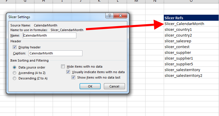
Replacing multiple slicer references with a single named range is easy to do. First, obtain the slicer names that you want to include in your formulas, and list them in a range within your scorecard.

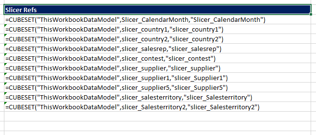
Now, you’ll need to create a CUBESET() formula for each slicer name, like this one:
=CUBESET(“ThisWorkbookDataModel”,slicer_CalendarMonth,”slicer_CalendarMonth”)
You’ll end up with your list looking like this (‘Show Formulas’ has been turned on to illustrate):

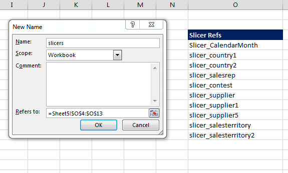
Next, highlight the list, click on the ‘Formulas’ tab and select ‘Define Name’. For this example, we’ll call our named range ‘slicers’.

Now, simply add the named range name within your CUBEVALUE() formula just like a slicer name.
=CUBEVALUE(“ThisWorkbookDataModel”,”[Measures].[Total Sales]”,slicers)
The true power and utility of this technique is revealed when your boss tells you to add or remove a slicer from the scorecard. All you do is modify your named range contents, and the entire scorecard updates!
D-Man, that was brilliant! Hats off to you, sir!
Tip 2: Use Named Sets for Cube Members
Not only did my sprawling scorecard have tons of slicer references, it also had many sets of the same cube members grouped together on rows, like this.

While developing my scorecard, I would need to modify each of these sets of region cubemembers on multiple tabs and check to make sure that they all matched. Oh the horror… the horror.
Solving this problem required a closer look at the CUBEMEMBER() and CUBERANKEDMEMBER() functions.
CUBEMEMBER() 101
CUBEMEMBER() formulas allow you to reference a specific ‘slice’ of a PowerPivot lookup or data table. For example, in a Calendar table, the CUBEMEMBER for the month of January would be CUBEMEMBER(“ThisWorkbookDataModel”,”[Calendar].[Month].[All].[January]”).
Because CUBEMEMBERS() are a slice of your model, they can be referenced within a CUBEVALUE() formula to return a measure result just for that slice. A great best practice is to use a CUBEMEMBER() formula as a row value, and then reference the cell containing your CUBEMEMBER() function within your CUBEVALUE() formulas. Using this technique makes for great scorecard tables.

Getting CUBEMEMBER()’s in Order with Named Sets and CUBERANKEDMEMBER()
A great way to manage a set of cube members is to build a named set and reference that set within a CUBERANKEDMEMBER() function. Named sets allow you to specify which cube members are to be included in a list, and also what order they should be in. This brings two benefits:
a.) Portability: The named set can be modified, and any range that references the named set will update not only the contents, but also the order of those cube members.
b.) Consistency/Accuracy: Only a single reference to the named set is needed. You won’t have to worry about inconsistencies in different CUBEMEMBER() formulas across multiple tabs.
Let’s Build a Named Set!
To create a named set, just insert a pivot table from Power Pivot and add the column with the cube members that you want to group together. For this example, I needed certain regions from the region table, so I pulled in the regions column.
Next, click on the ‘Analyze’ tab under Pivot Table Tools and select ‘Create Set Based on Row Items’. Add or remove the cube members that you want in your scorecard report, and arrange them in the order desired. Don’t forget to give your named set a snappy name! (I landed on ‘MySet’… wahoo… live dangerously!)

Next, to pull the named set into your scorecard, use CUBERANKEDMEMBER(), like this:
=CUBERANKEDMEMBER(“ThisWorkbookDataModel”,”[MySet]”,ROW(A1))
The last part with ROW(A1) just specifies that you want the set shown in the same order that you defined in your named set (ie rank 1, rank 2 etc).
Just like making updates to the slicer named range, you can now modify the contents or order of the members in your named set, and your scorecard cubevalue tables update automatically wherever the set is used! Want to move Region 1 down two rows in every table in the scorecard? No need to modify every single group of CUBEMEMBER() formulas, just click the down arrow in the named set manager and your entire scorecard updates!

Two Simple Tricks – One Awesome Data Tool
By using named ranges to consolidate slicer references and named sets to define a group of cube members, Excel developers can benefit from the flexibility of cube formulas, while still maintaining order and easy upkeep in their creations.
Just when you think you know it all, Excel proves it still has a whole lot of awesome up its sleeve! The fact Excel is so ubiquitous, yet it still offers gems like this to be discovered speaks to its depth as the world’s best data tool.
Get in touch with a P3 team member