
OK, if you recall from part one, we had a “year over year” time machine calculation going on, and it was built against a data set that lacked a “real” calendar table. Very cool. Very resourceful. And very necessary.
But the time machine had two problems. Let’s fix them.
Problem #1: Meaningless Grand Total
Let’s start with the easy one:

It is meaningless to have a “grand total” value for a measure that returns “last year’s sales.” What year would that BE, actually? It’s nonsense. So we use an old trick, one of the many flavors of IF(VALUES()):
=IF(COUNTROWS(VALUES(Periods[Year]))>1,BLANK(),
CALCULATE([Total Sales],
ALL(Periods),
FILTER(ALL(Periods), Periods[Year]=MAX(Periods[Year])-1),
VALUES(Periods[MerchPeriod])
)
)
Where the new IF “wrapper” is highlighted and the original formula is in normal font.
For more on that “IF VALUES” technique, please see this post.
The results are as desired, the grand total is now blank:
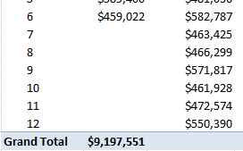
Problem solved. Moving on…
Problem #2: 2011 isn’t complete but we’re getting all of 2010 sales
Remember, our sales data for 2011 only goes through the first 6 months. So we do NOT want “last year sales” for months 7-12:
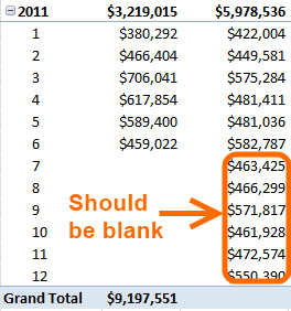
That can be solved a number of ways. The simplest is just to add another IF(), and have the Last Year Sales measure return BLANK() whenever there are no Sales:
=IF(COUNTROWS(VALUES(Periods[Year]))>1,BLANK(),
IF([Total Sales] = BLANK(), BLANK(),
CALCULATE([Total Sales],
ALL(Periods),
FILTER(ALL(Periods),
Periods[Year]=MAX(Periods[Year])-1
),
VALUES(Periods[MerchPeriod])
)
)
)
That trims the results to just the months desired:
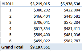
But note that the subtotal for 2011 is still too high:
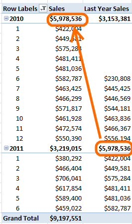
2010 Sales Through the First Six Months
This one is trickier. I struggled to find a good answer before coming up with the following:
Step 1: Add a “Next Year Period Num” Column to the Periods Table
Recall that my Sales table has a “Period Num” column that is the basis for the relationship with the Periods table:

And that matches up with a similar column in the Periods table:
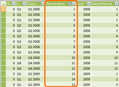
Note that Period Num does NOT reset to 1 with each new year (unlike MerchPeriod). So that is the absolute unique ID for a given Month/Year combo.
Well, I created a new column in the Periods table that tells me, for a given Period Num, what the equivalent Period Num will be NEXT year:
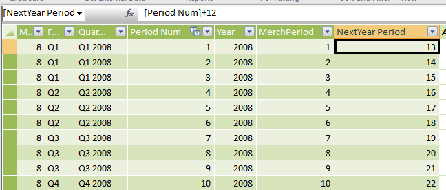
Now, in my FILTER statements, I can choose to match on THAT column instead.
Bringing it Home
OK, now that I have that column, I can add a new FILTER clause to my measure:
=IF(COUNTROWS(VALUES(Periods[Year]))>1,BLANK(),
CALCULATE([Total Sales],
ALL(Periods),
FILTER(ALL(Periods),
Periods[Year]=MAX(Periods[Year])-1
),
FILTER(ALL(Periods),
Periods[NextYear Period]<=
MAXX(
VALUES(PeriodSales[Period Num]),
PeriodSales[Period Num]
)
),
VALUES(Periods[MerchPeriod])
)
)
OK, what does that do? Simply put, it further filters the Periods table to NOT go beyond any periods for which we currently have records in the Sales table.
And the results:

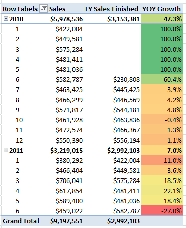
And now if you want YOY Growth, it’s straightforward:
=([Total Sales] - [LY Sales Finished]) / [Total Sales]
Which yields:
Measure in PowerPivot With a Custom Calendar
OK, I cheated and wrapped another IF(COUNTROWS(VALUES)) around the outside of the formula so that the grand total cell is blank again, because again, that’s a meaningless value to report. Details.
Isn’t that a lot of work?
Depends on how you look at it. First of all, it’s a lot harder to grasp the first time than it is as you get used to it, trust me.
But even better, this investment pays off forever. Normal Excel formulas may be easier to write the first time, but then you have to re-write and adjust them forever, every time your data changes. And every time your desired report shape changes.
This one is a portable formula. It goes wherever you want it to go, and eats whatever data you feed it. Forever. It’s worth a little extra effort.
OK but do I really have to understand all of that?
No, not really. Not right away. Think of it this way: this is what I do all day, every day. And I can tell you that figuring this out is not something you want to do in your spare time.
But once someone gives you the pattern? Wash, rinse, repeat. Make small adjustments as needed.
Honestly, that whole formula above could be wrapped up in a function provided by Microsoft, and all of the nasty stuff hidden. I told them as much last time I visited Redmond. And if it were a function rather than a formula, we wouldn’t care at all how it worked.
So… treat this as a pattern. Copy/paste and modify to fit your needs. Seriously.
Unfinished Business
I actually WILL retrace my steps here though and explain a number of things though, so that you CAN understand. I have a couple of posts in the queue aimed at just that.
Were there alternate ways to write this measure?
Yes, there were, especially in that last step where I needed to get the “Last year sales” measure correct for the 2011 subtotal. I could have used SUMX to make the year subtotal equal to the sum of its underlying months. That is worthy of a post for sure.
But I was wondering if there was still another way. A way that doesn’t use SUMX and doesn’t require a new calc column.
And for that, we need the Italians. So I’m gonna try out my new toy, the Boot Signal:

Get it? *Boot* Signal?
Get in touch with a P3 team member