Post by Rob Collie

Does Your Pivot Look Like This? Does its Slow make you Sad? Time for a Fix!
Tell me if this sounds familiar…
Yes, you know that pivots are meant to show aggregations. Summaries. Pivots were NOT invented to display thousands of rows of detail data.
But still, sometimes you need to do precisely that. The biz needs its list of customers and how much they’ve been buying, for instance, and all that data is in YOUR Power Pivot model.
And hey, pivots are really the only game in town* for table-shaped display of data. So, you build one of the monstrosities like the above.
(*OK yeah, you DO know about this thing called DAX Query Tables, but those are seriously a pain to set up. So, no. You rule those out before even starting. Just like me!
So You Do The Flattened Pivot Dance, Right???
In pictorial form…
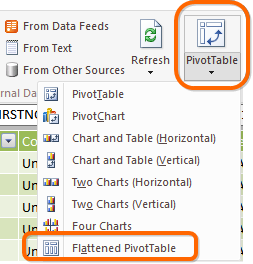
The Flattened Pivot Option – Found in the PivotTable Dropdown in the Power Pivot Window
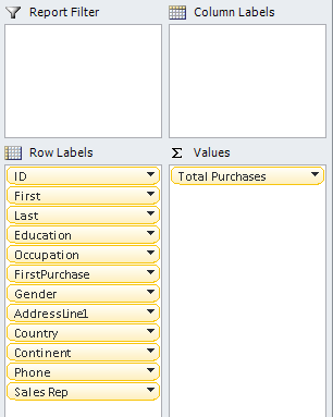
Next, You Pile a Whole Bunch of Fields Onto Rows
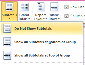
Then, on the PivotTable Design Ribbon Tab, You Turn Off All Subtotals
And Voila! It’s Slow as Heck.
Depending on the number of fields on rows, the number of tables involved, and the row counts and amount of uniqueness in those tables and fields, your flat pivot can range anywhere from “a little slower than average” all the way up through “this pivot will not finish calculating before our Sun goes Red Giant on us.” (Actually I think that certain pivots might literally meet that latter definition. More on this later.)
In my example, I have small row counts (every table has less than 100k rows), so even though I have 12 Row fields from 3 different tables, my pivot is simply annoying-slow, not galactic-slow.
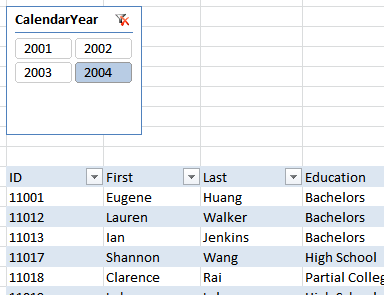
This Slicer Click Took 11 Seconds.
(But In Larger Data Sets, a Pivot Like This Can Take Hours.)
Why Is it Slow? The Short Version, Please? Please?
Here, let’s zoom in on the upper right corner of the pivot:
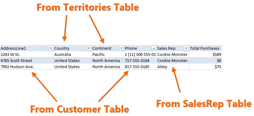
The Five Row Fields Pictured Come From Three Different Tables
Hey, that first customer, let’s call them customer XYZ, lives in Australia, has an Australian-style phone number, and has Cookie Monster for a Sales Rep. All well and good.
But Power Pivot doesn’t “know” that.
Behind the scenes though, the Power Pivot engine tried, um, a LOT of other combinations. For good measure (ho! good measure! get it??), it calculated a combination of customer XYZ, Germany for a country, North America for Continent, and Abby for a Sales Rep. Oh, and with a British phone number belonging to customer QRS to boot.
In fact, Power Pivot calculated EVERY SINGLE COMBINATION*. It just turns out that, hey, most of those combinations result in no data – there just isn’t any sales data for a country named Germany in a Continent named North America. So the engine sends back a BLANK() result, and the pivot doesn’t display blank results by default. You don’t SEE it, but trust me, it crunched it. While you waited.
This can literally result in the engine having to perform MILLIONS of “silly” calculations for every “real” calculation. And millions is when you’re lucky. It can get into Billions pretty quickly.
(*OK, I am not sure if Power Pivot tries nonsensical combinations within the same table. So between all the fields in the Customers table, it might be smarter and not do all the silly extra work. But across tables, definitely – it tries every permutation.)
An Aside… NECJ Unmasked!

Back in 2003 I was basically a high-functioning child, and I was in Denmark on Serious Business. In my job at Microsoft, I had been placed in charge of the BI features in the next release of Excel, aka Excel 2007.
So naturally, I had to go learn about BI. A guy named Allan Folting was my “tour guide” for this trip, because he a) was from Denmark b) knew a hell of a lot more about BI than I did and c) he reported to me. There were Bona Fide BI Customers to be found in Denmark, and Allan knew where they were.
On one of those visits, Allan and the customer started talking about Non-Empty CrossJoins. I had no idea what that meant, but I could tell by the way they pronounced it that it was Not Good. The customer was unhappy.
Since this sounded Bad, I asked Allan later to explain. He used a bunch of words. I made a half-hearted attempt to understand and then gave up. I was dedicated to my craft back then.
Anyway, I now know, in hindsight, that THIS topic – detailed pivot reports where the engine “boils the ocean” to find a single grain of sand – is the NECJ issue they were discussing. The rows that the pivot actually displays? You know, the meaningful ones? Those are the Non Empty rows. The multiple tables? That’s the CrossJoin part. We even have the CROSSJOIN function in DAX, which I used for Pokemon analysis last year, and then for real business purposes just this past week actually.
This is a trend in my life actually – Older Rob going “aha, THAT’s what they meant when Younger Rob was spacing out!” I think I just took a lot longer for me to mature, honestly. I even lost my baby teeth a lot later than average. I hope this means I live to be 120. And yes, Excel 2007 turned out great. I had a great team, and I actually was pretty good at my job. I’d just be better today.
OK. Here’s a Fix That May Help You.
Don’t put a bajillion fields on Rows. Put ONE field on Rows, and then use Measures for the rest.

Interesting Eh?
And the pivot still looks kinda the same…

This Pivot is Conveying the Same Information as the First One…

…But THIS Slicer Click Took 3 Seconds Instead of 11.
(And in more complex cases, it would be MUCH more than 4x faster.)
The Approach and Formulas
First, determine what each row of your report is supposed to show.
If each row is a single Customer, for instance, you MUST put a unique identifier for Customer on Rows. In this case I used the CustomerID column. (And if each row is a Product, well, you need a unique id for Product).
Then, for fields from the same table as the ID (Customers table in this case), the measures are simple-ish:
First:=FIRSTNONBLANK(Customers[FirstName],1)
Last:=FIRSTNONBLANK(Customers[LastName],1)
Etc. etc. for all the other fields in the Customers table we care about, like Phone and the like.
And remember, those only work if you have a unique identifier on Rows of the pivot!
Fields from Other Tables
That simple FIRSTNONBLANK formula isn’t going to work for the other tables, like Territories.
Since the Customers table has no relationship to Territories, the unique customer id column has no filtering power over Territories. So the FIRSTNONBLANK will operate on an unfiltered Territories table, and just give you the alphabetical first value from the entire table. That’s not what we want.
So here’s what I’ve done for Country and Continent, from the Territories table:
Cntry:=
  CALCULATE(FIRSTNONBLANK(Territories[Country],1),
            FILTER(Territories, [Total Purchases]>0))
Cont:=
  CALCULATE(FIRSTNONBLANK(Territories[Continent],1),
            FILTER(Territories, [Total Purchases]>0))
The FILTER strips the Territories table down to rows that have data in the Sales table (as represented by our [Total Purchases] measure). And since we only have one Customer in our filter context for each row of the pivot, that means we only get Territories rows where that Customer was active. In this case, that means we get their home country and continent.
Added Benefit: Sorting Works!
Let’s go back to our first pivot, the one with all the fields on Rows.
And now let’s sort the pivot Largest to Smallest by the Total Purchases amount…
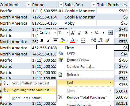
Let’s Sort This Sucker!
And the results…
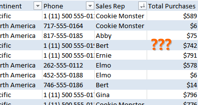
The Sort Operation Completed. But NOTHING Changed.
What the heck happened? Well, the pivot DID sort the Sales Rep field largest to smallest. See the little arrow on the dropdown button next to “Sales Rep” in the picture above? But since each Sales Rep value is being sorted “within” all of the other fields, each single value of Sales Rep is being sorted against itself. Which moves nothing.
You CAN work around that, by going to the dropdown button on the ID column of the pivot instead, choosing More Sort Options, and going from there to sort ID descending by the measure. That way you get what you want.
But what if you want to sort by First Purchase? You are flat out of luck. Seriously, you’re stuck if you’re using Row-based flat pivots and want to sort by any of the “property” columns other than the ID itself.
In the measure-oriented pivot though? You’re in BIZNESS…
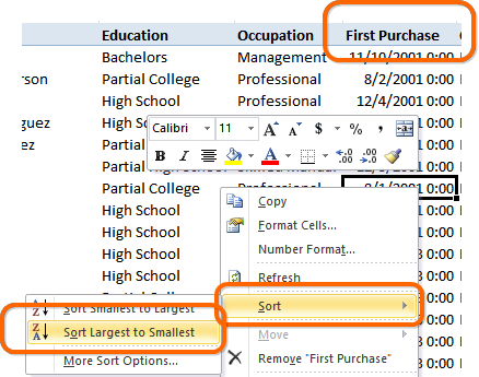
Absolutely, You Can Sort by First Purchase in the Measure-Oriented Pivot!
This results in the most recent first-purchasers floating to the top…

Results. We Like.
Yeah, OK, I’m cheating a bit here. This post is called Text Measures, and I just sorted by a Date measure. Excel pivots can’t sort accurately based on true text measures for some reason. The option is there, but it gives me weird results, at least in 2010:
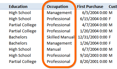
I Just Sorted by the Occupation Measure. But it’s not doing the right thing.
Oh well, can’t win ‘em all.
Get in touch with a P3 team member