By Avi Singh [Twitter]
This post is based on a query that I got in our monthly Q&A session held for our Online Class attendees.
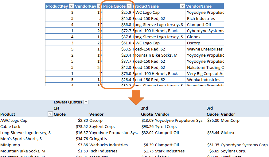
Input = Multiple quotes for different Products from different Vendors
Desired Output = For each Product show the top three quotes, both price and the Vendor name

Go from a list of Price Quotes to showing the lowest Vendor Quotes for each Product
A bit more on the Q&A session before we dive in. All our Online Class attendees are invited to a monthly Q&A session, in order to support them in their Power BI journey. Often what you learn in class, you would only apply sometime later. With the Q&A session, if you run into issues or have any questions, you have the opportunity to bring it up and discuss with your instructor. You can sign up for our upcoming Online Live Class on August 3-4.
Step 1: Structuring the Tables
We would clean things up and import the data into separate data and lookup tables. This may seem superfluous for the sample data set, but a real data set could have a lot more rows in the data table and a lot more columns (attributes) for the lookup table. Hence separating the data table and lookup tables is always a good approach.
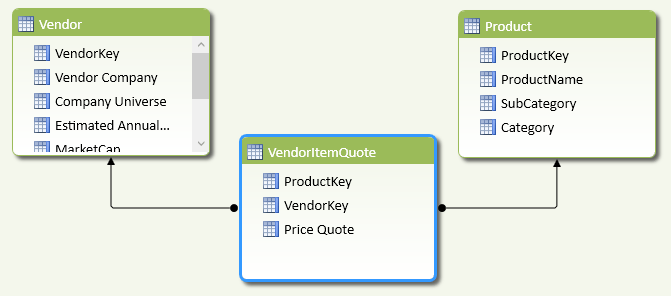
Our Vendor Quote data loaded as separate Data and Lookup Tables
Step 2: Brainstorm Approach to Writing Measure
When I first heard the problem I cycled through the following options:-
a) Simple Excel Pivot: I dismissed it almost as soon as it crossed my mind. If we simply drag Product and Vendor on rows and columns in a Pivot table, we get a picture but it’s not close to our desired output. I am sure there are ways to do this in Excel, but we need the magic of DAX Measures = “Define Once and Use Everywhere”. Where, we define them once and can use them in any pivot of any shape.

A simple pivot is unlikely to get us the desired output
b) Minimum Quote: My first thought was to determine the minimum quote
MinQuote:=MIN(VendorItemQuote[Price Quote])
And then write another measure find the next minimum quote and so on. But this felt like too much work. What if we had to show the top 10 Vendor quotes and not just top 3?
c) TOPN: Whenever I hear “top 3”, “top 10” etc. I gravitate towards the TOPN function. But this didn’t seem right either. TOPN would give me a set of top-ranked items from which I would still be left to determine the 1st, 2nd and 3rd.
d) RANKX: Next the RANKX crossed my mind and it felt like a jigsaw puzzle piece slid into place. So on we go with RANKX.
Step 3: Write RANKX Measure
Here is the anatomy off the RANKX function:-
RANKX(<table>, <expression>[, <value>[, <order>[, <ties>]]][, <expression>[, <value>[, <order>[, <ties>]]]]…)
Ascending/Descending Order: Here <order> can be
0 Descending Order (default)
1 Ascending Order
Typically, I skip the <order> parameter since the default (descending order) is what I’m looking for. So when determining my top customer, top product, top sales representative etc. the #1 rank would be with the highest value (e.g. the highest Sales).
But in this case, the lowest price quote is the best hence should be ranked #1. Therefore I would choose an ascending order (<order> = 1) for RANKX.
Attempt #1: Here is my first attempt, and there is a problem right away.
Rankx_Try1:=RANKX(ALL(Vendor), [MinQuote],,1)
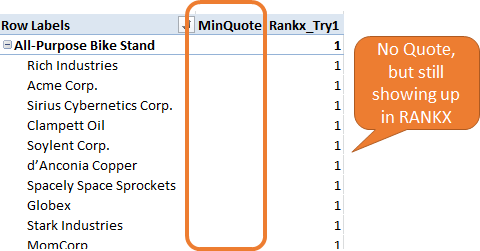
Even Vendors with no submitted quotes are showing up in RANKX result
All the vendors are getting ranked, even the ones which never submitted a quote for that product. Fine we will suppress the vendors without quotes in attempt #2.
Attempt #2: Suppress RANKX where no quotes.
Rankx_Try2:=IF(ISBLANK([MinQuote])
, BLANK()
, RANKX(ALL(Vendor), [MinQuote],,1)
)
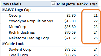
Oops! Ranking starts from #21 instead of #1 ??
This isn’t quite right either, since my ranking is not starting from #1, 2, 3 and so on. The Vendors which we just suppressed are still being factored in when RANKX is running; the suppression is after the fact.
I need to filter these out in the table RANKX is iterating over so that these are not considered to begin with. Remember RANKX is an iterator similar to other X functions (SUMX, AVERAGEX…). And we do so with this formula
Attempt #3: Only run RANKX on valid Vendor rows
VendorRankByQuote:=IF(ISBLANK([MinQuote])
, BLANK()
, RANKX(
FILTER(ALL(Vendor), NOT(ISBLANK([MinQuote])))
        , [MinQuote]
,
,1
)
)
The key difference is highlighted in bold. Now, instead of ALL(vendor) I am using FILTER to select only the Vendor rows with a valid quote. Here are the results:

RANKX is finally looking good!
Step 4: Writing the Final Measures for the Desired Output
Future Proofing Your Model: I often try to go beyond what is asked of me when building Power Pivot models. I try to think of not just what the customer has asked, but also what they might ask in the future. And I attempt to design my data model to be elegant and flexible enough to be able to answer new questions thrown its way. Over time I expect to tweak things a bit, write few new measures, but the core structure of the data model should remain stable. The only big changes being when we add new data sets – e.g. we start with the Sales data in your data model and then you bring in let’s say your Budget or Service Calls.
Back to our problem…In this case even though the user asked only for the top 3 quotes I chose to implement this using a disconnected table. This would allow me to easily extend this to top 5 or even top 10 quotes.
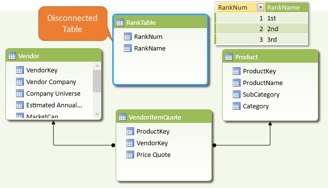
Adding a disconnected table to easily show Top N Vendor Quotes in a Pivot
We write a harvester measure to get the Selected Rank from our disconnected table, and then a new measure to get the corresponding Vendor Quote (based on SelectedRank).
SelectedRank:=IF(HASONEVALUE(RankTable[RankNum])
, VALUES(RankTable[RankNum])
, BLANK()
)
RankVendorQuote:=CALCULATE([MinQuote]
, FILTER(
Vendor
, [VendorRankByQuote] = [SelectedRank]
)
)
[SelectedRank] essentially returns 1, 2 or 3. Then we use FILTER to find the Vendor with the selected rank. Here are the results:-

The Top 1, 2, 3 Quotes shown in our Pivot
To be able to display the actual Vendor name the first write a helper measure and then our final measure on the same pattern as RankVendorQuote above.
SelectedVendorName:=IF(HASONEVALUE(Vendor[VendorKey])
, VALUES(Vendor[Vendor Company])
, BLANK()
)
RankVendorName:=CALCULATE([SelectedVendorName]
, FILTER(
Vendor
, [VendorRankByQuote] = [SelectedRank]
)
)

The Top 1, 2, 3 Vendors with the lowest quotes
Here is the pivot with both measures, getting us to the desired output:-

Our desired output with both measures on the pivot
Epilogue: Interestingly the person asking the question was asking me whether they should transform the data table itself using Power Query to get the desired output. This is becoming a very frequent question in our training classes, Q&A sessions and even our consulting work – which tool should I use? Should I use Power Pivot for Power Query for my task? I’ll save that one for my next blog post.
Power On!
-Avi Singh
Get in touch with a P3 team member