Parameterizing the report

In the Parameterized Report, how do I get the “Fan Pts” column on the far right of the cube formula report to respond to those parameter cells in the top left?

Easy.  The report is just formulas, so I can combine them with the parameter cells using Excel arithmetic.

Naming the Parameter Cells:  a Readability Convenience

The parameters themselves live in cells C3, C4, and C5.  I can reference them that way, but to make things easier to read, I’m going to give them names.

To give a name to cell C3, I select it.  Note the control at the upper left corner of the grid that displays the address C3:

I just click inside that control and start typing to give C3 another name.  In this case, I name it YardsPerRushPt, below:

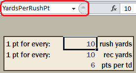
That will make my formulas easier to read, and also provides an added benefit later then I publish to SharePoint.

I then repeat this process for the other two parameter cells, C4 and C5, which I name YardsPerRecPt and PtsPerTD, respectively:

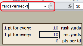
And

The Formula

The formula was always going to be easy to write, but now it will also be easier for us to read and understand.  Here is the formula in the Fan Pts column:

=CUBEVALUE(“Sandbox”,F3,Slicer_DayNightName,Slicer_WeekNbr,
“[Measures].[Rush Yards]“) / RushYardsPerPt

+CUBEVALUE(“Sandbox”,F3,Slicer_DayNightName,Slicer_WeekNbr,
“[Measures].[Rec Yards]“) / RecYdsPerPt

+CUBEVALUE(“Sandbox”,F3,Slicer_DayNightName,Slicer_WeekNbr,
“[Measures].[Rush TD]“) * PtsPerTD

All three CUBEVALUE terms are identical except for the measure they reference, and the parameter they either divide or multiply by – I have highlighted the differences in blue.

Note how I have used the cell names I defined above, rather than cell references.  This is an under-used and beneficial feature in Excel, and not at all specific to PowerPivot.

Dealing with #N/A – The Excel IFERROR() Function

Sometimes, a player will not have recorded any of a particular statistic.  This is especially true when you start slicing the report and the circumstances get narrower.

When that happens, Excel will often display #N/A in the cell instead of 0.  (In a future post I will delve into what determines 0 vs. #N/A).

Sometimes #N/A is ok to display.  But in the Fan Pts column, it’s a problem.  A player will often record yards but no TD’s, for instance.  But once a single term in the formula above goes to #N/A, the entire formula goes to #N/A, which is incorrect since that player DID have other statistics.

We just want #N/A terms to be treated as 0 in cases like this.  And the IFERROR() function in Excel is precisely designed for this.  If we wrap each term in IFERROR, we can specify an alternate value to be returned when an error like #N/A is encountered.

For example:

=IFERRROR(
CUBEVALUE”Sandbox”,F3,Slicer_DayNightName,
Slicer_WeekNbr,”[Measures].[Rush Yards]”)
/ RushYardsPerPt
,0
)

The IFERROR wrapper is highlighted in blue.  If no error is encountered, then the “meat” inside the IFERROR function (the CUBEVALUE divided by RushYardsPerPt) is returned as usual.

IFERROR is a very useful function overall, and all PowerPivot Pros should get to know it (a phrase that conjures memories of Jon Lovitz on SNL).  It can also be used to return custom strings in place of errors like “No data recorded.”

GET to know me!

Parameters Exposed in SharePoint-Published Reports!

Time for that “extra” benefit of named cells.  In my last video, remember how there was that expandable task pane rendered in Excel Services, that allowed me to change the parameter values interactively?

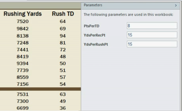
I said that required no coding, and that’s the truth 🙂  To activate that feature, you have to tunnel down a bit in the Excel UI, because hey, only hardcore folks like readers of this site would ever need such a thing, right?

First you go to the File tab in Excel and choose the “Share” option:

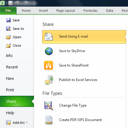
Then pick the “Publish to Excel Services” suboption, and click the button of the same name that I have highlighted:

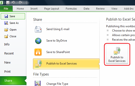
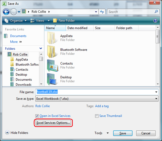
The dialog that comes up looks exactly like the Save As dialog.  And that’s what it is.  But there’s a new button there, highlighted below.  Click it!

Almost there, don’t give up!  There are two tabs on the resulting dialog.  The default tab, the Show tab, is very useful, but let’s skip that for now and switch to the Parameters tab:

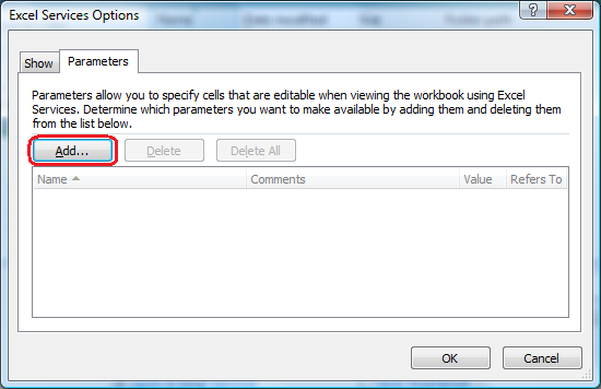
Clicking the highlighted “Add” button yields the following, final dialog in the chain:

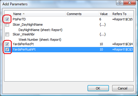
Every named range in the workbook appears here as a checkbox.  (Slicers are treated as named ranges, too, so that they can be referenced in formulas as well).  I select all three of the names representing my parameters, and then tunnel back out, clicking OK as I go.

(I can then save the file locally or save it to SharePoint, or cancel the Save As dialog and do a normal save later – in each case, the parameter settings will now be saved).

When I view this report on SharePoint, using the browser, the parameters pane will now appear automatically.

Parameters as Web Part Interface

The parameters pane is the simplest way to leverage these exposed parameters.  But those three cells are now also exposed as part of the web part framework, enabling other controls in SharePoint to send input values to the report.

That’s an advanced topic and only mentioned here in case you happen to be a SharePoint programmer as well 🙂

What Next?  Aren’t We Done?

Nope, we are not done.  We haven’t yet covered how to support dynamic sorting!  So that’s coming up.

And keep in mind that this whole foray into cube formulas is a bit of an advanced topic, and it gets trickier as you add more features into the report.  None of this is necessary for building PowerPivot reports – pivots are going to be your answer most of the time anyway.

Denny Lee, Your Time Has Come!

My esteemed colleague, Denny Lee, has found his way into the deep end of the pool lately with a [link removed due to 404] series of posts about Top N PowerPivot reports.

I have a lot of respect for Denny.  After all, the man can write MDX, and the existence of MDX is in some ways the reason why we had to create PowerPivot (…to replace MDX with something less intimidating).  And no one ends a sentence with “eh!” like Denny 🙂

But apparently Denny did not get the internal executive memo:  high-end Excel techniques are the domain of one Rob Collie, the P3 Adaptive !

Denny, you see, is now on my turf.  As they say in Excel power users circles, it’s, ahem, “on” now.

So my next few posts now have two purposes:  to explain how I did the dynamic sorting, and to give you some (cough cough, superior) alternatives to those MDX-backed techniques outlined by Denny.