Guest Post by Colin Banfield [LinkedIn]
After Rob posted Dynamic TopN Reports Using PowerPivot2!, I downloaded the workbook from the provided link to examine how his “tricks” were done. Shortly thereafter, I sent a message to Rob complementing the techniques he used, and mentioning the potential for using the techniques in other scenarios – especially those that include dynamic charts. I didn’t realize that I was setting myself up, because Rob asked if I’d be willing to write a post detailing one of these scenarios. For the sake of continuity, it makes sense to treat the scenario that I will be discussing as an extension of Dynamic TopN Reports via Slicers, Part 2. You should have thoroughly read and understood that post before you continue here.
The additions that I have made to Rob’s TopN reports are as follows:
- Created BottomN measures for Customers
- Created TopN/BottomN measures for Products
- Added a Year-Month slicer
Created TopN/BottomN charts for customers and products that react to slicer selections for TopN, By (selected measure), and Year-Month range.
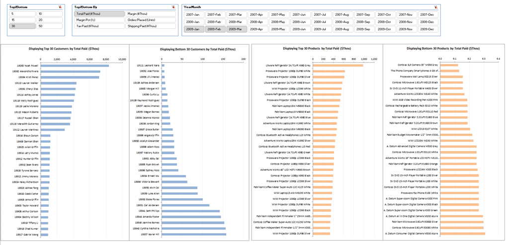
The final result of these efforts is shown in Figure 1.
First, a note on sample data
By far the biggest issue I faced in preparing the model was finding appropriate data for meaningful BottomN measures. The AdventureWorks and Contoso data warehouses are filled with one-off sales at the bottom, all with exactly the same sales amount. This situation makes it difficult to show any kind of variation in the BottomN charts. In the end, I decided to use the top 100,000 sales records from the Contoso data warehouse, summarized by date, customer, and product. For the customer and product dimensions, I pulled only the customer and products contributing to the Top 100,000 sales, and for the date dimension, I pulled complete dates for the years in the top 100,000 sales. As luck would have it though, except for a single customer, it turns out that the names for the customers contributing to the top 100,000 records are completely blank in the Contoso warehouse! Grrr. For a quick and dirty solution, I pasted the relevant customer IDs in an Excel worksheet, and pasted a list of names next to the IDs. I then linked the resulting table into PowerPivot.
New Measures
In Part 2, Rob provided the following top rank formula (I’ve added “Top” to the original name):
[CustomerTopRankBySelections] =
RANKX(ALL(Customer[FullName]), [Selected TopN Value], ,0)
The additional standard rank formulas are thus:
[CustomerBottomRankBySelections] =
RANKX(ALL(Customer[FullName]), [Selected TopN Value], ,1)
[ProductTopRankBySelections] =
RANKX(ALL(Product[ProductName]), [Selected TopN Value], ,0)[ProductBottomRankBySelections] =
RANKX(ALL(Product[ProductName]), [Selected TopN Value], ,1)
For controlling the PivotTable Value Filter, Rob provided the following formula (Once more, I’ve added “Top” to the original name):
[Should Top Customer Be Included] =
IF([CustomerTopRankBySelections]<=[SelectedTopNNumber],1,0)
The additional formulas are thus:
[Should Bottom Customer Be Included] =
IF([CustomerBottomRankBySelections]<=[SelectedTopNNumber],1,0)
[Should Top Product Be Included] =
IF([ProductTopRankBySelections]<=[SelectedTopNNumber],1,0)
[Should Bottom Product Be Included] =
IF([ProductBottomRankBySelections]<=[SelectedTopNNumber],1,0)
With the exception of some modifications we need to make to the standard bottom rank formulas (explainer later), the preceding are the only additional formulas required for the extended model.
The data for the four charts shown in Figure 1 comes from four copies of the PivotTable that Rob created in part Part 2. However, instead of displaying all of the dynamic measures in a single PivotTable, each PivotTable contains a single dynamic measure, which is the following measure Rob provided:
[Selected TopN Value] =
SWITCH([Selected TopN Measure],
1, [Total Paid],
2, [Margin],
3, [Margin Pct],
4, [Orders Placed],
5, [Tax Paid],
6, [Shipping Paid]
)
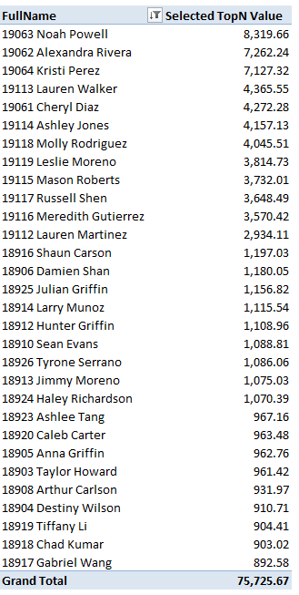
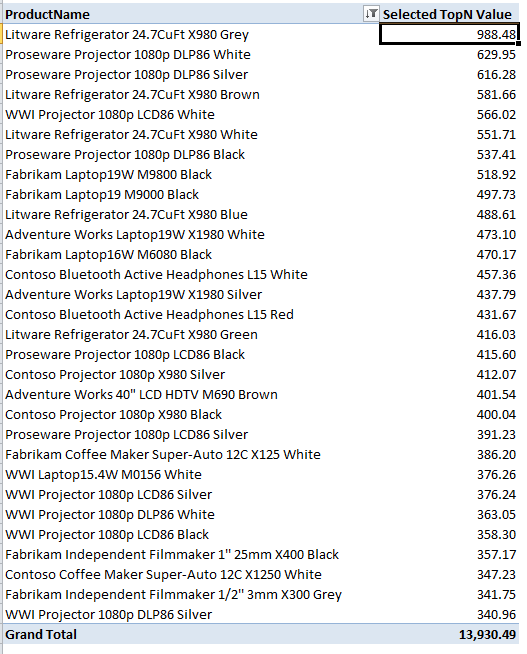
The actual measure used is thus governed by the selection made in the “TopN/BottomN By” slicer. In addition to this measure, each PivotTable is sliced by either product or customer, as shown in Figure 2.
The charts work perfectly fine when the data is sliced by customer or product. As shown in Figure 1, I added a Year-Month slicer. Using the standard rank formulas previously given, when the data is filtered by Year-Month, there is no data whatsoever in the BottomN charts! This problem is occurring because when sliced by year & month, there are many customers and products with no sales in the selected timeframe (way more than 50 customer/products in the dataset I’m using). RANKX() includes all the empty sale values in the bottom ranking, and therefore gives all the empty sales a bottom rank of 1! When the Value filter in the PivotTable is applied, you end up with a blank PivotTable because all of the bottom 5, 10 ,20, 30, 50 values are blank.
You can see what’s happening by adding the rank measure to one of the BottomN PivotTables, as shown in Figure 3.

How can we solve this problem? First let’s modify the RANKX() formula to remove all the blank values. The formula for the BottomN products becomes:
[ProductBottomRankBySelections] =
IF([Selected TopN Value]>0,
RANKX(ALL(Product[ProductName]),
[Selected TopN Value],,
1
)
The result of this change is shown in Figure 4.
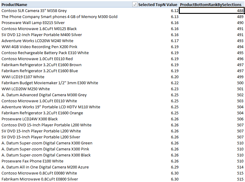
We now see the bottom ranks for products with data. They are sequential, but the ranks are far outside the values that I want to select in my TopN/BottomN slicer. It appears that Rob’s Value filter trick has hit a brick wall. The question is, how can we renumber the ranks starting from 1? Well, RANKX() has an optional “value” argument, which, if included in the RANKX() formula, returns the rank of value compared to other values in the dataset. Value can be a non-zero calculated value, or a hard-coded value. For example, if I set the value to 10, the formula returns the rank of value 10 compared to other values in the dataset. Setting the value argument thus overrides the individual rankings shown in figure 4. How we can use the value argument to our advantage is not immediately obvious. It turns out that if we set value to a any value equal to or less than the lowest non-zero value in our dataset, the formula returns the rank of the lowest non-zero value in the dataset. If we add the following measure to the PivotTable,
[LowestNonZeroRank] =
RANKX(ALL(Product[ProductName]),
[Selected TopN Value],
0.00001,
1
)
we get the values shown in Figure 5. In the figure, I’ve hidden rows so that you can see the boundary between empty-value rows, and rows with values.
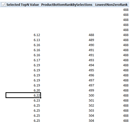
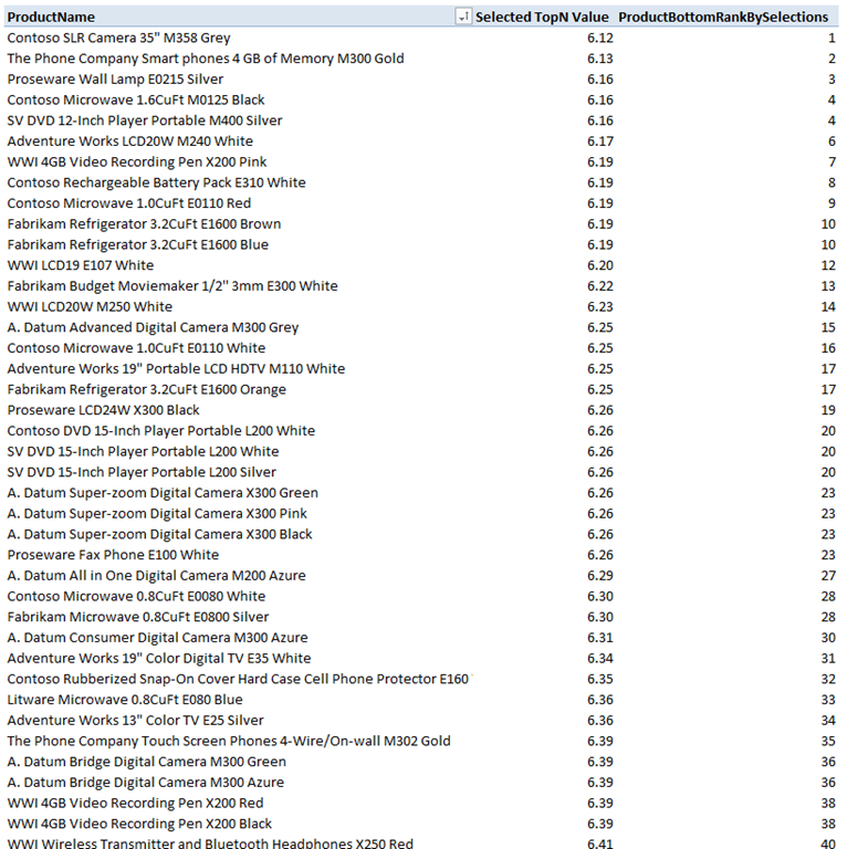
For any given dataset, 0.01 would represent the lowest likely sales value (one cent in US currency). The values in the above figures were scaled by 1000 (more on this later), so I used 0.00001, as this represents 0.01/1000. To restart the product ranks from 1, we subtract the LowestNonZeroRank from the individual product ranks and add 1. Also, since we have to add the additional complexity because of the Year-Month filter, we can build the measure so that we use the more complex expression when the Year-Month filter is applied, or the standard rank expression otherwise. The complete BottomN rank formulas are as follows:
[CustomerBottomRankBySelections] =
IF(HASONEVALUE(Customer[FullName]),
IF(ISFILTERED(CalendarDate[YearMonth]), ‘Use the following expression if the Year-Month filter is applied
IF([Selected TopN Value]>0,
RANKX(ALL(Customer[FullName]),
[Selected TopN Value],,
1
)+1
–
RANKX(ALL(Customer[FullName]),
[Selected TopN Value],
0.00001,
1
)
),
RANKX(ALL(Customer[FullName]), ‘Otherwise use this standard expression
[Selected TopN Value],,
1
)
)
)
[ProductBottomRankBySelections] =
IF(HASONEVALUE(Product[ProductName]),
IF(ISFILTERED(CalendarDate[YearMonth]),
IF([Selected TopN Value]>0,
RANKX(ALL(Product[ProductName]),
[Selected TopN Value],,
1
)+1
–
RANKX(ALL(Product[ProductName]),
[Selected TopN Value],
0.00001,
1
)
),
RANKX(ALL(Product[ProductName]),
[Selected TopN Value],,
1
)
)
)
I include HASONEVALUE for completeness sake. If subtotals or grand total are added to the tables, we want to display blank for totals and subtotal ranks.
The completed BottomN PivotTable for Product is shown in Figure 6 (for the corresponding chart, the rank column is removed).
Other Modifications
In the previous section, I briefly mentioned that some of the measures have been scaled. This was done to allow the chart value axes to accommodate dynamic measures with vastly different scales. The [Selected TopN Value] is thus modified as follows:
[Selected TopN Value] =
SWITCH([Selected TopN Measure],
1, [Total Paid]/1000,
2, [Margin]/1000,
3, [Margin Pct]*100,
4, [Orders Placed],
5, [Tax Paid]/1000,
6, [Shipping Paid]/1000
)
To display the scaling factors in the chart titles, I modified the MeasureForTopN table as shown in Figure 7.

Get in touch with a P3 team member