DAX – “CONTAINSX” Revisited: What WAS the Match?

Building on a Popular Technique

Last week’s post on “CONTAINSX” proved to be quite popular.  In the comments, Sasha provided an alternate formula that used FILTER instead of SUMX.  Honestly I have a been of a “fetish” for SUMX – after all it IS the 5-Point Palm Exploding Function Technique – so at first I was like “nice work Sasha but I’m sticking with my SUMX.”

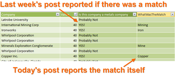
But then “en” asked if we could write a formula that reported what the matching keyword actually WAS – not just whether there WAS a match.

And then, Sasha’s formula came in super-handy.  A couple of quick mods and we were in business.  Read on for the formula, but first, a quick aside.

Another thing that is easier in Power Pivot than “Traditional” Excel

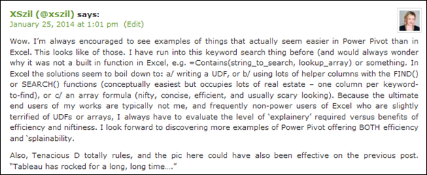
I really enjoyed the comments (and the emails) we received about the CONTAINSX post.  Here are two of my faves:

Excel Warrior Priestesses Endorse Power Pivot Over Traditional Excel for Problems Like These
(Although I Think She Was Talking About Today’s Followup Technique, not the Original)

“Freaking AMAZEBALLS” is Actually a Technical Term,
Known Only to Those on the Inside of the Data Revolution
(Identity Redacted to Protect Our Operators in the Trenches)

Personally I suspected that this was easier in Power Pivot than regular Excel.  And normally, calc columns are NOT the strength of Power Pivot (measures are the game changers).  But now I’ve grown so used to calc columns in Power Pivot that I often struggle to write the “old Excel” equivalent.  I’ve crossed over, and can no longer judge such matters for myself.

So it was very cool to hear from XSzil on that front.

And, of course, AMAZEBALLS for the win.

Get on with it!

OK, new formula time:

The formula for the highlighted column is:

[WhatWasTheMatch] =

=FIRSTNONBLANK(FILTER(
                      VALUES(MatchList[Keyword]),
                      SEARCH(
                             Matchlist[Keyword],
                             Companies[Company],
                             1,
                             0
)
)
,1
              )

Explanation – FIRSTNONBLANK Part (Yellow)

This is sort of a nonstandard use of FIRSTNONBLANK.  But then again, I find myself often “mis-using” FIRSTNONBLANK in useful ways like this.

You see the yellow-highlighted “,1” up there?  That is the second input to FIRSTNONBLANK, and in “standard” uses, that is typically a measure, and you’re trying to find, for instance, the first time a customer EVER bought something, which happens when the sales measure first returns a non-blank value.

But here, by using 1 as the last input, we “short circuit” the “is it blank?” test (the “NONBLANK” part), and grab the first value we find, period.

In other words, FIRSTNONBLANK with a 1 as the last input is a makeshift “FIRST TEXT VALUE WE FIND” function.

Explanation – the FILTER(VALUES(SEARCH(…))) part

OK, everything else (the green parts) has only one purpose – to return a single column of text values from the Matchlist[Keyword] column.  But only values from that column that actually were found in the current row of Companies[Company].

In other words, it’s only going to return keywords that were found.

But it all starts with VALUES(Matchlist[Keyword]).  And since there is no relationship or other dependency between the Companies table and the Matchlist table, this will ALWAYS start out with EVERY distinct value from the Matchlist[Keyword] column:

In this particular calc column formula, VALUES(Matchlist[Keyword])
Always starts with the unfiltered list of all values in that column.

Then the FILTER() kicks in and only keeps rows/values where the <filter expr> evaluates to TRUE.

Sasha cleverly used the SEARCH() function as the <filter expr> test to his FILTER().  I happily stole that.  Since SEARCH returns a non-zero number whenever it finds something, and FILTER treats nonzero numbers as TRUE, well, FILTER only keeps values that it finds.

OK Now What?

Last time I kinda left it to your imagination – what you would DO with such a column.

Well, how about slapping our new column on Rows of a pivot, with a couple of measures?

Our New Column Works Pretty Well on Rows Don’t You Think?

Pretty cool.  Note that I typed over the “Row Labels” cell in the pivot and called it Industry, and typed over the blank cell and called it “<unknown>.”  Just to make things a bit more “Fisher-Price” for the consumer of the report, ya know.

Other things you could do:

1. Use the new column as a slicer instead of a Rows field.
2. Use the new column as a <filter> input to a CALCULATE.  A new measure called [Average Value of Copper Companies], for instance, with formula CALCULATE([Average Value], Companies[WhatWasTheMatch]=”Copper”)
3. Write another calc column that groups “Mine” and “Mining” into a single value, like, um, “Mining.”  And then maybe use THAT new column for any of the purposes above.

Download the Updated Workbook

The updated workbook is available for download here.

Enjoy