Conditional Formatting with Different Thresholds per Test, per Product, per Store, per Division, etc.

 
After a long hiatus, David Hager has returned with a new guest post.  He has a clever Excel trick/formula for applying different conditional formatting “acceptable ranges” depending on the context of the current row.  In his work, different Tests have different acceptable ranges of values that qualify as Pass/Fail/Warning.

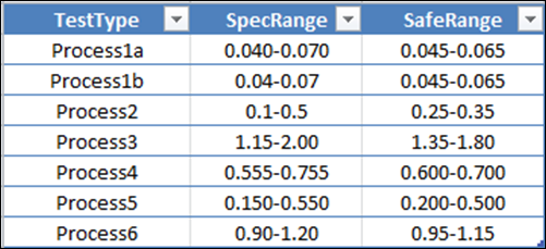
Each Test Has a Different “Pass Range” and “Safe Range” –
David Hager’s Technique Translates This Table Quickly into CF Rules

I think this technique can be extended to basically anything:  an acceptable sales growth figure for Store A may be different than that for Store B (or Product A vs. Product B, etc.)

His post also got me thinking about the new “KPI” feature in PowerPivot V2, so I will return later today with a brief follow-on post.

Conditional Formatting on a Case-by-Case Basis:  Status of a Test Result

Guest Post By David Hager

A test result usually has specifications, a window of acceptability, associated with it. Those specifications may be stored in a data table as text. An example would be “0.05-1.50”. In order to better target the middle of the specification range, there is a safety range that can be applied as well. An example based on the specification shown would be “0.07-1.30”. It is useful to be able to determine visually whether the test result is inside the safety range, outside the safety range but inside the specification range, or outside the specification range. The best way to do this in Excel is through the use of conditional formatting (CF). However, it may not be convenient to convert these specification strings to numbers so that they can be used in the CF formulas. Another consideration is being able to handle the correct rounding based on significant figures. The following formulas can be used with Excel’s CF feature to highlight test results based on a specification range.

The following picture illustrates the application of the CF on results in a table. In particular, note that although the values in B5 and B6 are the same, the number of significant figures for the spec in C5 affords a failed value vs. a passing value for B6.

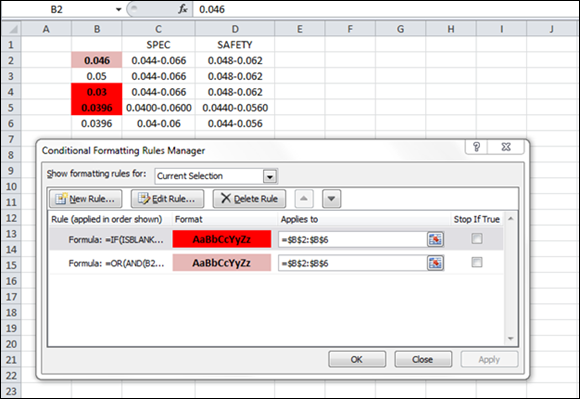
FIG. 1

The CF formula for indicating a result is outside of the safety range is:

=OR(AND(B2>=–LEFT(C2,FIND(“-“,C2)-1),B2<=–LEFT(D2,FIND(“-“,D2)-1)),AND(B2>=–MID(D2,FIND(“-“,D2)+1,10),B2<=–MID(C2,FIND(“-“,C2)+1,10)))

Since this formula provides formatting based on whether the result is in or out of the safety range, it is not critical that it contain the ability to operate on the number of significant figures present. It “looks” at the lower and upper ranges in the spec range that are not bound by the safety range and formats them appropriately based on whether the test result is in either of those ranges.

The CF formula for indicating pass or fail is:

=IF(ISBLANK(B2),FALSE,OR(MROUND(B2,1/(10^(LEN(LEFT(C2,FIND(“-“,C2)-1))-FIND(“.”,LEFT(C2,FIND(“-“,C2)-1)))))<–LEFT(C2,FIND(“-“,C2)-1), MROUND(B2,1/(10^(LEN(MID(C2,FIND(“-“,C2)+1,10))-FIND(“.”,MID(C2,FIND(“-“,C2)+1,10)))))>—MID(C2,FIND(“-“,C2)+1,10)))

Basically, this formula returns the characters before the dash and after the dash in the specification range and converts them into numbers (highlighted in green). The double negative sign works as a shortcut method of converting a text value into a number in Excel. They are compared against the actual test result, rounded to the number of significant figures inherent to the specs (highlighted in yellow). The 2^nd argument of the MROUND function returns a fractional number for the number of digits after the decimal point. If the test result is below the lower limit or above the upper limit of the spec range, the CF format is applied.

Initially, this article was going to be only about using these formulas in Excel as conditional formats. However, Rob forced me to provide a PowerPivot solution by agreeing that I could send him anything I wanted. Faced with this this kind of browbeating J, I turned to working on applying this concept in PowerPivot.

Two linked tables are needed to construct this model. In Figure 2, each test type is defined by its specification and safety range.

FIG. 2

In Figure 3, the table holds each test result along with the test type, the date and the test number.

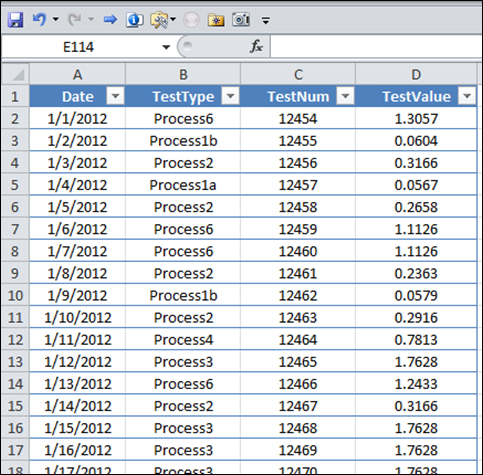
FIG. 3

After creating a relationship between the two tables in the PowerPivot window, three calculated columns were added to this table. The spec and safety range were added to the table (i.e. – =RELATED(ProcessSpecs[SpecRange])) and the test status, as shown in the following formula.

=IF(ISBLANK([TestValue]),”NoResult”,IF(OR(AND([TestValue]>=VALUE(LEFT([SpecRange],FIND(“-“,[SpecRange])-1)),[TestValue]<=VALUE(LEFT([SafeRange],FIND(“-“,[SafeRange])-1))),AND([TestValue]>=VALUE(MID([SafeRange],FIND(“-“,[SafeRange])+1,10)),[TestValue]<=VALUE(MID([SpecRange],FIND(“-“,[SpecRange])+1,10)))),“Warning”,IF(OR(MROUND([TestValue],1/10^(LEN(LEFT([SpecRange],FIND(“-“,[SpecRange])-1))-FIND(“.”,LEFT([SpecRange],FIND(“-“,[SpecRange])-1))))<VALUE(LEFT([SpecRange],FIND(“-“,[SpecRange])-1)),MROUND([TestValue],1/10^(LEN(MID([SpecRange],FIND(“-“,[SpecRange])+1,10))-FIND(“.”,MID([SpecRange],FIND(“”,[SpecRange])+1,10))))>VALUE(MID([SpecRange],FIND(“-“,[SpecRange])+1,10))),“Fail”,”Pass”)))

This DAX formula combines the two formulas that were used for conditional formatting. A change was needed to obtain the same functionality as the Excel formula. The DAX language does not permit the use of a double negative to convert text to a number, so the VALUE function was used in its place.

The pivot table shown in Figure 4 depicts one representation of the data. In this case, the test status is used as in a slicer to show all of the samples where the test result was in the warning (not in the safety range, but not failing).

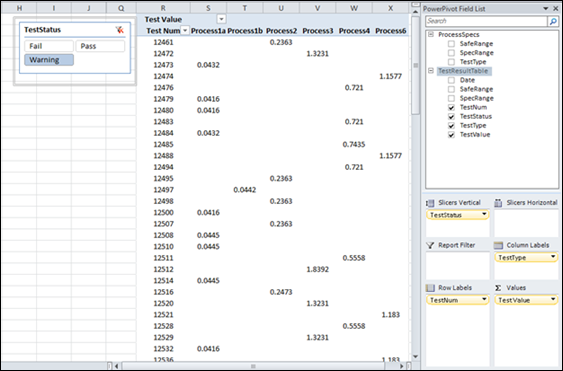
FIG. 4

The fake data created for this model did not initially include multiple results that were obtained for a specific sample. In order to demonstrate this, I added one additional result for test # 12461 to the bottom of result table. The result for this sample can be seen in Figure 5. I also need to point out that a real model would include the time for each test measurement, as well as a separate date-time table.

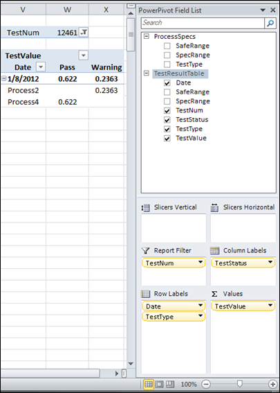
FIG. 5

As you can see, these “spec” formulas provide a powerful method of looking at test results in PowerPivot as well as their use in conditional formatting. The workbook used for this article can be downloaded here (note: this workbook was constructed in PowerPivot 2012/V2, so do not attempt to use in V1).

Note From Rob:  Translating into PowerPivot Conditional Formatting

As I mentioned at the beginning of the post, seeing this got me thinking that we should also be able to apply Pass/Fail/Warning as a conditional formatting rule in the pivot, and not just as a slicer.  And the new KPI feature in PowerPivot V2 might be helpful in that regard.

I will return later today with a quick follow-on post on my experiments in that space.