
What an amazing year 2018 has started out to be!
Joining the P3 Adaptive team was an aspiration of mine that started in the Fall of 2013… I wanted to BE a part of this team and this community – to be able to share what I have personally experienced and what I have learned about using PowerPivot In Excel and Power BI and how these tools can really CHANGE your life for the BETTER!
This year has kicked off with a lot of firsts for me!
In January, I shared my first blog posts with the P3 Adaptive community. That same first blog post was also featured on the Guy in A Cube’s Channel on YouTube, also a first! (… AND I beat my kiddo’s, who for years now, have aspired to be YouTubers!)
In February, I taught my first Power Query Public Training class, right here in Phoenix! Which surprisingly, many of the students had traveled to Phoenix to attend the training. Maybe they were expecting AMAZING training AND some WARMER weather?! Which I would have to say, Phoenix did disappoint a bit on the warmer climate this year. But come back now and stay through to Aug., Sept., and Oct. and Phoenix, for sure, will not disappoint! Possibly, it’s the only place in the country where we sweat in our Halloween costumes!
In March, I presented for the first time at PASS SQL Saturday event in Phoenix! PASS SQL Saturday is an event that is held once a year per city – it’s completely FREE to attendees (THANKS to the sponsors), and it’s a great way to spend a day learning about many technologies – including Power BI. The local Phoenix PASS chapter is an AMAZING group of people, and I can say without a doubt that I would never have fully made this career journey without ALL their help and encouragement. The ENERGY at the event and the EXCITEMENT of the many people attending from all areas of the business was PHENOMENAL! It was great being able to connect with people of similar interests, AND I even saw a few familiar faces from our P3 Adaptive – April 2017 – Public Training class in Chicago (which a year ago, was my first week after joining forces with the P3 Adaptive team!)
Also, in March, I was able to travel to Memphis, Tennessee for the first time – to share our On-Site 3-Day Power BI Training with a FANTASTIC and FUN group of people working in Supply Chain Management.
I’ve NEVER been to Memphis, and I didn’t know what to expect. I arrived at my travel destination EARLY for once (also a first since traveling for P3). The weather was quite chilly, windy and grey – no Bueno (Umm… I DO live in Phoenix for a reason!) But there were blue, yellow, and purple flowers and beautiful trees with white and purple blossoms – so it was warmer at one point. My Uber driver suggested that he drop me off to check in at the hotel and that he’d wait for me and drive me over to see Graceland. Now, I hadn’t planned on site-seeing… but sure, why not – you only live once! And WOW, I thought, this Uber driver is SO nice. He drove me by the wall outside of Graceland and dropped me off to take the tour!

Every interaction that I had with people here in Memphis was incredibly FRIENDLY, WARM and just overly NICE! The ENERGY of the town is different… it’s simple, kind and soulful. And so, after touring Graceland and reflecting on Elvis and his life… one might wonder if the ENERGY that was Elvis, if that ENERGY still lives on here with the people of Memphis? I’d say that I think it does.
So, in the spirit of Elvis, I want to blog today about a SIMPLE challenge that presented itself during the workshop portion of the On-Site 3-Day Power BI Training in Memphis.
USE CASE: Create a Power BI Dashboard using Excel Files from a Folder – SIMPLE and EASY enough!
“A well’a bless my soul.”
SOLUTION: Use Power Query to Combine Excel Files from a Folder – been there DONE that!
“What’sa wrong with me?”
CHALLENGE: To the naked eye, the Excel Files looked to be the same. But when loaded into Power Query, one of the Excel files imports differently and is messing up the combine process!
“I’m NOT in love, I’m all shook up!”
STEP 1: Open the Excel Files and LOOK at the data – same/same. One BLANK row, one Header Row,
one Column Header Row and then the data (or so we thought!)
Exhibit A Exhibit B

STEP 2: Open PBID
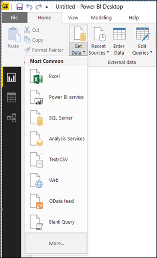
From the Home table, select Get Data > then More… from the drop-down list.
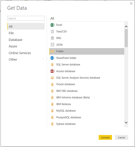
In the Get Data window, select the Folder option (to Combine multiple Excel files from a Folder).
Select the Browse… button to path to the Folder location of where the Excel Files are located <or> just type the Folder path location and select the OK Button.

The next window displays all the files that are in the Folder. Select the Combine down arrow button.
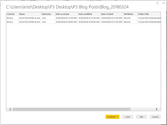
Then select the Combine & Edit option.

STEP 3: So far so good!
And since I’ve read Matt Allington’s “Understanding Power Query Combine” blog post (THANK YOU very much Matt!) https://exceleratorbi.com.au/understanding-power-query-combine/
… I now understand the whole Combine Files MAGIC that happens, and I’m not scared or confused ANYMORE by these next steps where Power BI simply wants an Example File to use as a parameter to then build logic that creates a function to be used for the MAGICAL Combine process!
(Before 2016, we used to have to do this a different way!)
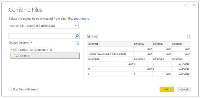
But WAIT just a minute… why is this happening?

In the preview, Exhibit A does NOT have an extra line before the Header Row, but Exhibit B DOES have an extra line before the Header Row – well, that is strange!
NOTE: I’m TELLING all of YOU this right now …but it wasn’t initially apparent that THIS was the ROOT cause of the problem. If you have many files with ONE file and this problem, it might be hard to find!
If I use Exhibit A as the Example File, and then continue by selecting the OK button – the final Combined data set in the Other Queries folder contains a couple of problems.

Problems:
- I don’t have my Column Header names; I have the default Column1, Column2, Column3, etc.
- I have a Row that is EXTRA
- And I need to remove that Header Row, but the Header Row name isn’t the same!
If I use Exhibit B as the Example File, I still end up with the same problems ;(
Okay, well… I know I can go to the Transform Sample File step, add additional steps in the Applied Steps and any changes that I make in the Sample will be applied to ALL Excel files in my Folder.
- Select the Transform Sample File step

- If I were to use Exhibit A as the Example file, I could Remove Rows > Remove Top 1 Rows followed by Use First Row as Headers, and this works well against the Exhibit A file!

However, since the Exhibit B file contains an EXTRA row for some reason… this logic causes a problem when we get to Exhibit B.

“Happy ending, happy ending
Give me a story with a happy ending.”

… Well, if you remember back from Step 3, the problem IS that extra row in Exhibit B. And I only SEE this extra row when I’m in the Power Query editor – I did not see it in Excel with my naked eye. What we need is a SIMPLE solution now that we know the root cause!
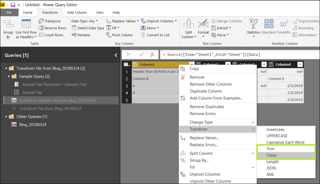
STEP 4: Let’s highlight all the columns (CTRL+A) then use Transform > click Format drop-down > then select Clean! Followed by Transform > click Format drop-down > then select Trim!
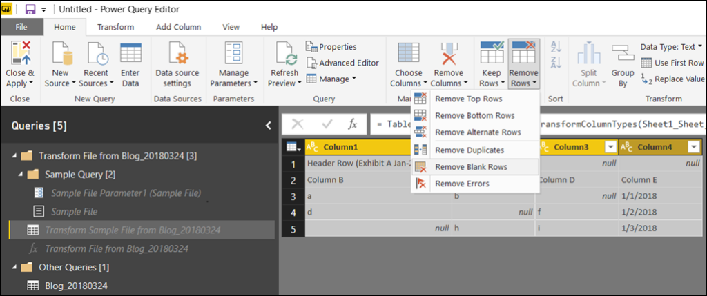
STEP 5: Now we can use Home > Remove Rows > and Remove Blank Rows (now that the CLEAN and TRIM have been applied!)
STEP 6: Finally, select Home > Use First Rows as Headers. And it works!

And with that… THANK YOU Memphis, I enjoyed my time here and the SIMPLE dirty data challenge.
… Elvis has left the building!

Microsoft’s platform is the world’s most fluid & powerful data toolset. Get the most out of it.
No one knows the Power BI ecosystem better than the folks who started the whole thing – us.
Let us guide your organization through the change required to become a data-oriented culture while squeezing every last drop* of value out of your Microsoft platform investment.
* – we reserve the right to substitute Olympic-sized swimming pools of value in place of “drops” at our discretion.
Get in touch with a P3 team member