Guest post by David Churchward
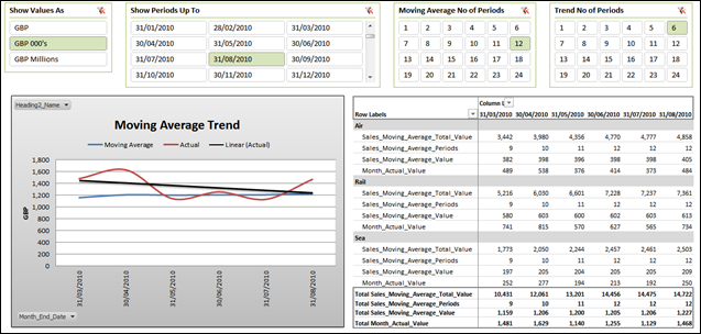
I’ve always been a firm believer that moving averages probably give a better insight into trends within a business than a simple trend line associated to a set of values such as monthly sales (although I tend to review these two values together). The reason for this is that a trend can be skewed by one or two values that may not be representative of the underlying business such as spikes associated to seasonality or a specific event. When BillD highlighted a query regarding this concept in his comments on Profit & Loss (Part 2) – Compare and Analyse, I thought it would be a great idea to flex our P&L dataset to provide some Moving Average capability.
In this post, I will explain what moving averages are intended to deliver and explain how to calculate them using the sales elements of the example data used in the Profit & Loss series of posts. I will then add the flexibility for users to select the time frame that the moving average calculation should consider, the number of trend periods to be displayed and the end date of the report.
What is a Moving Average?
The most common moving average measure is generally referred to as a 12 month moving average. In the case of our sales data, for any given period, this measure would sum the last 12 months of sales preceding and including the month being analysed and then divide by 12 to show an average sales value for that timeframe. In financial terms, the equation is therefore quite simply:
12 Month Moving Average = Sum of Sales for Last 12 Months / 12
This all seems very straight forward but there’s a lot of complexity involved if we want to put the Moving Average timeframe (represented as 12 in the above example) in the hands of the user, give them the power to select the number of trend periods to be displayed and the month that the report should display up to.
The Dataset
The dataset that we’re using looks something like below.
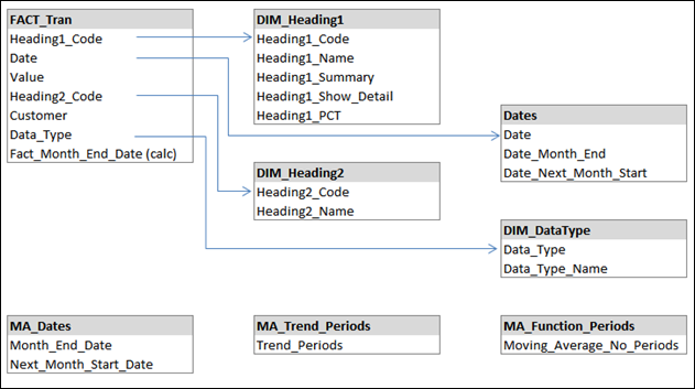
Note – I’m using PowerPivot V1. Design viewer is available in V2 but I’ve hashed this together – nothing clever!
You’ll notice that FACT_Tran (our dataset to be analysed) is linked to DIM_Heading1, DIM_Heading2 and DIM_DataType to provide some categorisation to our dataset. I’ve also linked to Dates which is a sequential set of dates that more than covers the timespan of our dataset. This table carries some static additional information based on the date:
Date_Month_End = EOMONTH(Dates[Date],0)
Date_Next_Month_Start = Dates[Date_Month_End]+1
Once again, we’re not quite registering on Rob’s spicy scale! Rest assured that you’ll be getting a more intense DAX workout as we go on.
As these date measures aren’t expected to be dynamic, I’ve coded them in the PowerPivot window. This allows them to be calculated on file refresh but they won’t need to recalculate for each slicer operation which removes performance overhead from our ultimate dynamic measure.
For reasons that I’ll come on to later, I also need the month end date on my fact table as I can’t use the Month End Date on my Dates table in my measures. I can however pull the same value across to my FACT_Tran table using the following measure:
Fact_Month_End_Date = RELATED(Dates[Date_Month_End])
So What Are These Unlinked MA_ Tables?
The reason for these tables should become apparent as we go on. In brief, they’re going to be used as parameters or headings on our report. The reason that they exist and that they’re not linked to the rest of our data is simply because I don’t want them to be filtered by our measures. Instead, I want them to drive the filtering.
Initial PivotTable Setup
I’m going to be displaying a series of data organised in monthly columns. The user will be given slicers to set Month End Date (the last period to be shown on the report), Number of Periods for Moving Average (this will ultimately be part of our divisor calculation) and Number of Periods for Trend (this will be the number of monthly columns that we will display on our trend). We can establish these slicers straight away and link them to the pivot.
I obviously need a month end date as a column heading but which one? To some extent I’ve given this away earlier on. In short, I need to use my MA_Dates[Month_End_Date] field. The reason is that this field isn’t linked to our dataset and therefore won’t be affected by any other filters. If I use a date field that is part of my dataset or part of a linked table, the values available may be filtered down by the users selections. I can get around this using an ALL() expression to give me the correct values, but the problem is that the column is still filtered and my results will all be displayed in one column. It’s difficult to explain until you see it so please go ahead and try – it’s worth hitting the brick wall to really understand it!
Calculating Sum of Sales for Last X Months
The first part of our equation is to calculate the total value for sales across all periods within a dynamic timeframe to be selected by the user. For this I use a Calculate function that looks like this:
CALCULATE(
[Cascade_Value_All],
DIM_Heading1[Heading1_Name]=”Sales”,
DIM_DataType[Data_Type_Name]=”Actual”,
DATESBETWEEN(
Dates[Date],
DATEADD(
LASTDATE(VALUES(MA_Dates[Next_Month_Start_Date])),
MAX(MA_Function_Periods[Moving_Average_No_Periods])*-1,MONTH
),
LASTDATE(VALUES(MA_Dates[Month_End_Date]))
)
)
I’m using a base measure called Cascade_Value_All that was created in Profit & Loss – The Art of the Cascading Subtotal. I’m then filtering that measure to limit my dataset to records that relate to Sales and a data type of Actual (ie eliminating Budget). This is simple filtering of a CALCULATE function. However, it gets a bit more tasty with the third filter which limits the dataset to a series of dates that are dependent on the users selections in slicers and our date column heading.
The DATESBETWEEN function has the syntax DATESBETWEEN(dates, start_date, end_date) and works like this:
- I set the field that requires filtering (Dates[Data]). I’ve found that this works best if this is a linked table of sequential dates without any breaks. If you have any breaks, there’s a chance you might not get an answer as the answer that you evaluate to has to be available in the table.
- My start date is a DATEADD function that calculates the column heading date less the number of months that the user has selected on the “Moving Average No of Periods” slicer. I use the LASTDATE(VALUES(MA_Dates[Next_Month_Start_Date)) function to retrieve the Next_Month_Start_Date value from the MA_Dates table that relates to the date represented on the column heading. I then rewind by the number of months selected on the slicer using MAX(MA_Function_Periods[Moving_Average_No_Periods])*-1. The “-1” is used to go back in time. The reason I use Next_Month_Start_Date and a multiple of –1 is more clearly explained in Slicers For Selecting Last “X” Periods.
- My end date is simply the Month_End_Date as shown on the column heading of the report. This is calculated using LASTDATE(VALUES(MA_Dates[Month_End_Date]).

That’s great, but my measure isn’t taking any account of my “Show Periods Up To” selection and the “Trend No of Periods” that I’ve selected. We therefore need to limit the measure to only execute when certain parameters hold as true based on these selections. I only want values to be displayed when my column heading date is:
- Less than or equal to the selected Month End Date on my “Show Periods Up To” slicer AND
- Greater than or equal to the selected Month End Date LESS the selected number of periods on my “Trend No of Periods” slicer.
To do this, I use an IF statement to determine when my CALCULATE function should execute. Let’s call this measure Sales_Moving_Average_Total_Value
Sales_Moving_Average_Total_Value
= IF(COUNTROWS(VALUES(MA_Dates[Month_End_Date]))=1,
IF(VALUES(MA_Dates[Month_End_Date])<=
LASTDATE(Dates[Date_Month_End])
&&VALUES(MA_Dates[Month_End_Date])>=
DATEADD(
LASTDATE(Dates[Date_Next_Month_Start]),
(MAX(MA_Trend_Periods[Trend_Periods])*-1),MONTH),
CALCULATE(
[Cascade_Value_All],
DIM_Heading1[Heading1_Name]=”Sales”,
DIM_DataType[Data_Type_Name]=”Actual”,
DATESBETWEEN(
Dates[Date],
DATEADD(
LASTDATE(MA_Dates[Next_Month_Start_Date]),
MAX(MA_Function_Periods[Moving_Average_No_Periods])*-1,MONTH
),
LASTDATE(VALUES(MA_Dates[Month_End_Date]))
)
)
)
)
The IF statement works as follows:
- I first need to determine that I’m evaluating only where I have one value for MA_Date[Month_End_Date]. If I don’t do this, I get that old favourite error in my subsequent evaluation that says that a table of multiple values was supplied……
- I then evaluate to determine if my column heading date (VALUES(MA_Dates[Month_End_Date]) is less than or equal to the date selected on the Month End Period slicer (LASTDATE(dates[Date_Month_End])…AND (&&)
- My column heading date is greater than or equal to a calculated date which is X periods prior to the selected “Show Periods Up To” as selected on the Slicer. I use a DATEADD function for this similar to that used in my CALCULATE function except we’re adjusting the date by the value selected on the “Trend No of Periods” slicer.
With this in place, we have the total sales for the selected period relating to the users selections.

So my table is now limited to the number of trend periods selected and represents the month end date selected.
So Now We Just Divide By “Moving Average No of Periods” Right? eh NO!
We’ve calculated our total sales for the period relating to the users selections. You would be forgiven for suggesting that we simply divide by the number of moving average periods selected. Depending on your data, you could do this but the problem is that the dataset may not hold the selected number of periods, especially if the user can select a month end date that goes back in time. As a result, we need to work out how may periods are present in our Sales_Moving_Average_Total_Value measure.
Sales_Moving_Average_Periods
= IF(COUNTROWS(VALUES(MA_Dates[Month_End_Date]))=1,
IF(VALUES(MA_Dates[Month_End_Date])<=
LASTDATE(Dates[Date_Month_End])
&&VALUES(MA_Dates[Month_End_Date])>=
DATEADD(
LASTDATE(Dates[Date_Next_Month_Start]),
(MAX(MA_Trend_Periods[Trend_Periods])*-1),MONTH),
CALCULATE(
COUNTROWS(DISTINCT(FACT_Tran[Fact_Month_End_Date])),
DIM_Heading1[Heading1_Name]=”Sales”,
DIM_DataType[Data_Type_Name]=”Actual”,
DATESBETWEEN(
Dates[Date],
DATEADD(LASTDATE(MA_Dates[Next_Month_Start_Date]),
MAX(MA_Function_Periods[Moving_Average_No_Periods])*-1,MONTH),
LASTDATE(VALUES(MA_Dates[Month_End_Date]))
)
)
)
)
This measure is essentially the same as my Sales_Moving_Average_Total measure. The only real difference is that we count the distinct date values in our dataset as opposed to calling the Cascade_Value_All measure. I mentioned earlier that there was a reason why I needed the month end date to be held on my FACT_Tran table and this is why. If I use any other table holding the month end date, that table isn’t going to have been filtered in the way that the core dataset has been filtered. As an example, my Dates table has a series of dates that spans my dataset timeframe and more. As a result, evaluating against this table will deduce that the table does in fact have dates that precede my dataset and there is therefore no evaluation as to whether there is a transaction held in the dataset for that date.

As you can see, since my dataset runs from 1st July 2009, I only have 9 periods of data to evaluate for my 31/03/2010 column. If I had divided by 12 (as per my “Moving Average No of Periods” slicer selection), I would have got a very wrong answer. Obviously, this is slightly contrived but it’s worthy of consideration.
And Now The Simple Bit
I can understand that the last two measures have taken some absorbing, especially working out when particular date fields should be used. For some light relief, the next measure won’t really tax you!
Sales_Moving_Average_Value =
IFERROR(
[Sales_Moving_Average_Total_Value]/[Sales_Moving_Average_Periods],
BLANK()
)
This is a simple division with a bit of error checking to avoid any nasties.
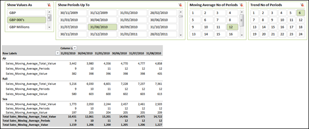
When It’s All Put Together
Since all of these measure are portable, I can create another Pivot Table on the same basis as the one above (with Sales_Moving_Average_Value given an alias of Moving Average), move some stuff around, add a measure for the actual sales value for the month (I won’t go into that now, but it’s a simple CALCULATE measure with some time intelligence) and I then reconfigure to look like the following:
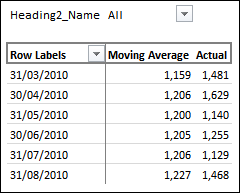
I can then drive a simple line chart and apply a trend line to my “Actual” measure with the chart conveniently hiding my data grid that drives it.
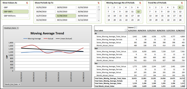
As you can see, a trend on my Actual measure shows a steady decline. My Moving Average, however, shows a relatively stable, if not slightly improving trend. Seasonality of some other spikes are obviously therefore involved and the reality is that both measures probably need to be reviewed side by side.
For those of you reading this who are interested in seeing the workbook of this example, I’ll look to post this in a future post when I take this analysis one step further to cover the whole P&L. Sorry to make you wait.
I hope this helps you out BillD…
One More Point to Note
Those eagle eyed DAX pros out there have probably noticed that my IF functions only contain a calculation to evaluate when the logical test reaches a True answer. The reason is that the function assumes BLANK() when a false evaluation condition isn’t provided. I haven’t worked out if there’s any performance impact using this method on large datasets. It’s up to you what you chose to do and if anyone can convince me why coding the False condition as BLANK() is best practice, I will quickly change my habits!
Get in touch with a P3 team member