DAX – The Magic of IF(VALUES())

“I’m Dan Marino, and IF() anyone knows the VALUE() of protection, it’s me.”

Boom!  An Ace Ventura quote finally graces the blog.  Yes folks, that fine work of American cinema did indeed feature Dan Marino reprising his real-world ad for Isotoner.

(UPDATE:  I had the val_if_true, val_if_false arguments reversed in my sample formulas, even though I had them correct in Excel.  I’m rusty .  Fixed now.)

But more importantly, I wanted to revisit this little two-function combo:  IF(VALUES()).  I’ve covered it before a few times, but generally in the context of covering something else.

And since this is one of my favorite techniques, I think it deserves its own dedicated post.  A series of posts, actually.  Let’s dig in.

In Measures, You Can’t Just use IF()!

In regular Excel, the IF() function is a familiar tool to most of us:

      IF(logical_test, value_if_true, value_if_false)

In PowerPivot, you can use precisely that same version of IF() in calculated columns.  So, for example:

      IF(Table1[Column1]>6, 0, 1)

In a measure formula, however, you cannot do that.  If you do, you will receive the following error:

To better understand why that happens, let’s get ourselves an example…

“Whoa, did you say DimDown???”

Yeah that’s right, the Great Football Project is back after a long hiatus! I had a phone call yesterday with a Pittsburgh Steelers fan.  You know Pittsburgh?  It’s a drinking town with a football problem.

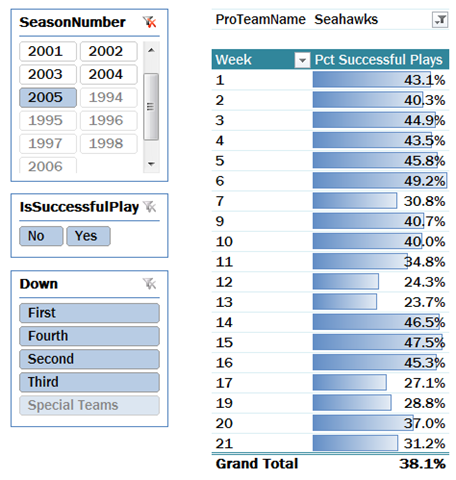
Anyway, he requested a return to the football project, under the umbrella of “how do the Steelers win another Super Bowl?”  Given that I lived in Seattle for 13 years, and witnessed his Steelers literally “steel” a Super Bowl from Seattle via lopsided referee calls, I decided that we should look at what should have been the Seahawks’ championship season:  2005.

[Pct Successful Plays] is a measure that I’ve been developing with Hugh Millen.  I’m not going to reveal the “secret sauce” behind said measure, but you can see that in Week 21, when the Seahawks played Pittsburgh in the title game, only 31.2% of their plays were successful – well under their 38.1% total for the year, and their 6th-worst percentage of the year.

Applying Different Formulas in Different Circumstances

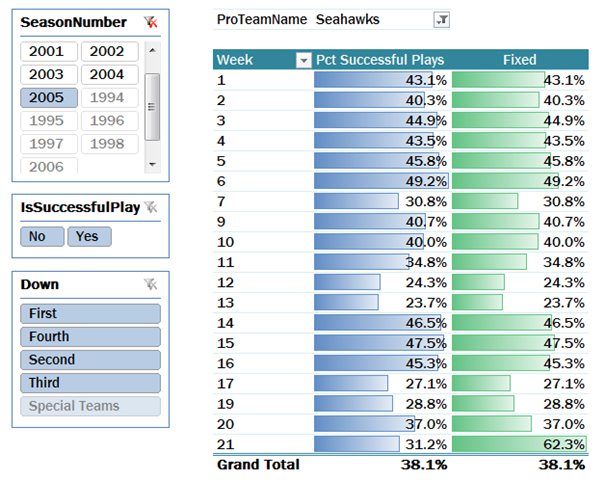
Now let’s say that I want to return a different value for this measure in Week 21, which is Super Bowl week.  You know…  I want to “correct” for bad referee calls.

I’ll create a new measure, [Corrected Pct Successful Plays].  In normal cases, I want that measure to just return the same value as would be returned by the original [Pct Successful Plays] measure.

But in week 21, I want to double it.  Just to set things straight.  (In real business, there are many legitimate examples of this technique, like applying a different formula in the West region versus the East region of a sales territory).

If I just use IF() by itself, I will get the error I showed in the previous section.

But if I nest VALUES() inside of the IF(), it will work!

      IF(VALUES(Schedule[WeekNbr])=21, [Pct Successful Plays]* 2,
       [Pct Successful Plays] )

Neat, huh?  Returns the same value as [Pct Successful Plays], except it doubles in Week 21.

A Return to the Golden Rules of DAX Measures:  No Naked Columns!

So why is VALUES() required?  Because you cannot have “naked” columns in your measures.  This is one of the “golden rules” for DAX measures that I first introduced over a year ago – see this video for an explanation.

If you’re not interested in watching that video right now, fine, just take my word for it:  in most places, you cannot just include column references in your measures, you have to wrap them in a valid function.  (And go watch the video later, as it’s a concise explanation of the fundamentals of DAX measures, and something I cover on every consulting/training engagement).

VALUES(Table[Column]), however, IS legal in a measure, and VALUES returns the list of values for the specified column in the current context.  So in the last row of the pivot above, it returns 21, and the formula becomes IF(21=21, 2 * [Pct Successful Plays], [Pct Successful Plays]).

Make sense?  OK, good, because I am lying to you.  There’s one more trick I have to show you, as the formula above actually STILL doesn’t work.

But…  IF(VALUES()) only works when there is only a single value!

OK, here’s the formula from above, repeated here:

      IF(VALUES(Schedule[WeekNbr])=21, [Pct Successful Plays] * 2,
       [Pct Successful Plays])

On each individual row of the pivot above, [WeekNbr] DOES have a single value (1, 2, 3, …  21).

There are actually many cases, however, where [WeekNbr] does NOT have a single value.

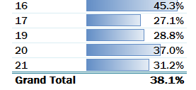
For instance, in the Grand Total cell of the pivot:

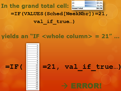
In the grand total cell, [WeekNbr] is NOT a single value.  It is actually ALL weeks.  In that case, the VALUES function returns a full column of values, and comparing a whole column to a single value doesn’t work out too well.

I like to visualize that problem in my head:

      IF(VALUES(Column)) yields an error when there is more than one value of Column

And by the way, that’s not an error that you will just see displayed in the pivot’s grand total cell.  It will “tank” the evaluation of the entire pivot:

Protecting against multi-value situations

Protecting against this is pretty simple.  You just use another IF() to “guard” your IF(VALUES()).

The “guard” if is highlighted below, wrapped around the original formula in normal font.

=IF(COUNTROWS(VALUES(Schedule[WeekNbr]))=1,
        IF(VALUES(Schedule[WeekNbr])=21, [Pct Successful Plays] * 2,
         [Pct Successful Plays]), 
   [Pct Successful Plays])

In essence, you never let your IF(VALUES()) get evaluated unless there is only one value!  If there is more than one value (as there is in the grand total, or in a subtotal), the formula above just returns the original measure (that’s the “[Pct Successful Plays]” at the end).

Making it simple (seriously, just follow the pattern!)

A lot to digest?

It may seem bad, yes.  But you don’t actually have to grasp it fully.  You can just treat this as a “pattern” that you use.

For example, here is the formula turned into a pattern.  You just substitute your columns and values in the highlighted spots:

  =IF(COUNTROWS(VALUES( <Your Column Here> ))=1,
        IF(VALUES( <Your Column Here> ) =  <Test Value Here> ,
         <Result if True> ,
         <Result if False> ),
   <Result for subtotals and grandtotals> )

The stage is set for some serious fun!

OK, with all of that covered, that sets us up for a series of quick, simple, and powerful techniques that I can share in the next blog post.