Today I had a huge source table that looked like this:
| Store | Month | Payment Type | Some Number |
| A | Jan | Cash | 10 |
| A | Jan | Credit | 12 |
| A | Jan | Debit | 13 |
| A | Feb | Cash | 14 |
| A | Feb | Credit | 17 |
| A | Feb | Debit | 9 |
| B | Jan | Cash | 21 |
| B | Jan | Credit | 12 |
| B | Jan | Debit | 6 |
That went on for about 100K rows. Thing is, I didn’t care about the Payment Type, and never would. (My data set was a little different than this, so it’s hard to explain why I’d never care).
What I wanted was a much smaller source table that collapsed the PaymentType column and aggregated Some Number:
| Store | Month | Sales |
| A | Jan | 35 |
| A | Feb | 40 |
| B | Jan | 39 |
Which would end up being about 1% of the rows.
My first thought was to create another table in PowerPivot and then use formulas to aggregate data from the big table into the new, small table.
But how to populate the first two columns of that new table? Just getting all of the distinct pairs of Store/Month was going to be tedious work – I had > 200 stores! I was contemplating VBA macros.
Then it hit me: Flat Pivots! (Kasper and I had been talking about them today for another reason – I think he’s going to share that soon).
What’s a Flat Pivot?
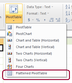
It’s a new feature in Excel 2010. Once you insert a PivotTable, you can set it to appear flat.
Thing is, I forget how you do that, because PowerPivot makes it SUPER easy at Pivot creation time, as shown here at right.
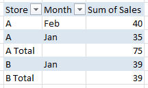
Drag Store and Month onto Rows, and heck, throw Sales into the Values area! That yielded a PivotTable like this one below:


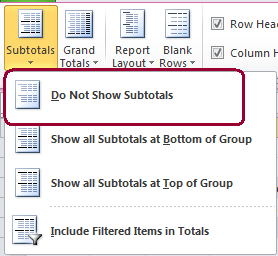
Gotta get rid of those pesky subtotals now. On the Design tab of the ribbon is the button I need:

Which yields this as my Pivot:

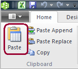
Paste button:
Copy that to the clipboard and switch back over to the PowerPivot window.
On the main ribbon tab, click the big fat

That yields a new table in PowerPivot:

It has all the unique combos of Store/Month, AND it already has the aggregated numerical column! No formulas needed.
Took about 2 minutes. Keep this in mind, it will save you a TON of time someday.
Hey, your PowerPivot Window is Green!!!
Why yes. Yes it is. Jealous? Cough cough, GREEN with envy?
Don’t go looking for the setting. It’s not there yet. This is an improvement in recent builds of the addin. You might also have noticed that the PowerPivot ribbon visuals are a little crisper.
Coming soon to a desktop near you 🙂
Get in touch with a P3 team member