Dax: Back to the basics

Figure 1 View outside of my home office window May 2^nd, 2018 Fairbanks, Alaska.

Intro

Hello, my name is Matthew Brice and I am guest broadcasting from my home office (via tape delay) in Fairbanks, Alaska.  PPPro put out a call for guest bloggers and they were kind enough to allow me to provide some content.  It has been a long time putting it together as I started in May as the pic above suggests.    Have no fear as the snow did eventually melt.

The power in Power BI comes from the Dax language. I read a lot of forum posts on both the Power BI community and Mr. Excel sites, and in my observation, it seems that beginners don’t fully grasp the core concept on which Dax is built. This post is my attempt to explain it my way.

At its core, all of Dax can be summed up in one sentence:

Dax is about manipulating the values that are filtering columns in the data model.

That’s it. Every function we write in Dax is used to change these values. Now, while the concept is simple, writing the code requires an in-depth understanding of the nuances of Dax (which is beyond the scope of one blog post).

Here I will try to provide a 10,000-foot view of Dax to aid in seeing the forest through the trees, and hopefully as a useful reference to guide your way.

Filter Context

For me, whenever I am new to a concept, and I read a statement like the one above, I often say “Well that’s great, but just what does that mean?” I am a big believer in mental models or ways of visualizing the flow of execution. As most are aware, all the values filtering columns are collectively known as the filter context[1]. I visualize filter context as a separate box that sits “on top” of the tables in the data model. We then use Dax to add/remove/change the values in the box before being applied to the model and computing our value. Simple right? To make the example clear, we will only talk about a very straightforward model (in fact just a single table). But the concept is the same no matter how many tables are in the model.

*The trick with the larger models is following the flow across relationships.

Here is our raw dataset:

Figure 2  Raw Table Data

Below I have Table 1 as a pivot table.

Table 1 Raw Data

The yellow highlighted value shown has the filter context in my filter context box.

Where “Sum of Amount” is a simple :

Sum of Amount := SUM ( Table1[Amount] )

To arrive at the value of 100, we sum up all the values in the Amount column where Person = “Anne,” Color = “Blue” and Type = “Bike.” When we filter the data source table with these values, we are left with a single row to sum. We see that our expected value of 100 is returned in the pivot.

That is simple enough, but what if we want to do a more complicated calculation?  To do that we must dive into functions that add/remove/change values in our filter context box.

CALCULATE

The most common and arguably the most important function in Dax is CALCULATE.

It’s function reference is:

CALCULATE(<expression>,<filter1>,<filter2>…)

CALCULATE is somewhat unique in that it evaluates the 2nd, 3rd, …nth parameter first, and evaluates the first parameter last using values from my Filter Context Box. I think it is extremely helpful to list briefly the steps CALCULATE performs whenever it is invoked. (So maybe we are not at 10,000 feet, but 5,000?)

The CALCULATE function performs the following operations:

1. Create a new filter context by cloning the existing one. (***Important visual step!***)
2. Move rows in the row context to the new clone filter context box one by one replacing filters if it references the same column. (We will ignore this step for this post)
3. Evaluate each filter argument to CALCULATE in the old filter context and then add column filters to the new clone filter context box one by one, replacing column filters if it references the same column.
4. Evaluate the first argument in the newly constructed filter context.
5. Destroy this newly created, cloned filter context box before moving on to calculating the next “cell.”

It is much easier to visualize with an example:

So suppose we wanted to ignore the color of the item when summing up the values.  In Dax we would write the following measure:

Sum of Amount No Color =
CALCULATE ( SUM ( Table1[Amount] ), ALL ( Table1[Color] ) )

This measure reads “Sum the values according to the Filter context box, but first remove any filters on the column Table1[Color]”.

Let’s look at the result first, then step through how the Dax engine calculated the value.

As you can see here, the highlighted field is 400.

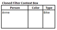
1. Clone the existing filter context (Edit/Copy/Paste if you will):

2. Move Row context into Filter context (ignore for this post)

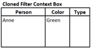
3. Evaluate CALCULATE parameters. In this case, our only parameter is ALL ( Table1[Color] ) which removes any filter on the ‘Color’ column, so our Filter Context box is now this:

4. Evaluate the first parameter with our Cloned Filter Context box. When you apply the Person = “Anne” and Type = “Bike,” the remaining rows to sum up look like this and voila the sum of the rows is 400.

Note: Remember, the preceding steps were only to calculate the highlighted cell.  Once completed, the Dax engine logically moves to the next cell in the pivot and goes through the algorithm again.

5. Destroy the Cloned Filter Context Box.

It’s simple once you understand the steps! 

Now let’s create a new measure with an added parameter.

Sum of Amount No Type Ben only: =
CALCULATE (
    SUM ( Table1[Amount] ),
    ALL ( Table1[Type] ),
Table1[Person] = “Ben”
)

 This measure reads “Sum the values according to the Filter context box, but remove any filters on the column Table1[Type] and only keeps the rows where the column Table1[Person] = “Ben”.”

Again, we will look at the strange looking result first and then step through how the Dax Engine computed the value.

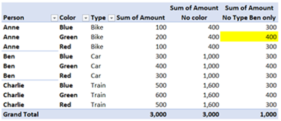
Once again we use the CALCULATE algorithm:

1. Clone the existing filter context
2. Move Row context into Filter context (ignore for this post)
3. Evaluate CALCULATE parameters.  Since we have two parameters, we have two steps to do:
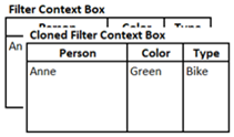
   1. ALL(Table1[Type] ) This removes any filters on the Table1[Type] column so now the Cloned Context Filter Box looks like this:
   2. Table1[Person] = “Ben”[1]. This step says to remove any existing filters on the column Table1[Person] and  then add the filter “Ben.” After doing so, our Cloned Filter Context Box looks like this.

4. Evaluate the first parameter with our cloned Filter Context. When you apply the Person = “Ben” and Color = “Green,” there remains only one row, and so the value returned is 400.

5. Destroy the Cloned Filter Context Box.

So even though on the pivot it shows “Anne,” “Green” and “Bike,” we used Dax to change the column filters to return the sum of the values for “Ben” & “Green” only.

Finally, for our last example we’ll change the CALCULATE statement to be like so:

Sum of Amount Green only :=
CALCULATE ( SUM ( Table1[Amount] ), FILTER ( Table1, Table1[Color] = “Green” ) )

Here is what the table looks like with this measure added:

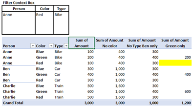
So for the highlighted cell, we’ll do the same drill as the last two examples:

 4 Evaluate the first parameter with our cloned Filter Context.  When we apply the filter Person = “Anne” and Color = “Red” AND Color = “Green” (meaning each row in Table1 must have a case where Color is Red and Green at the same time) and Type = “Bike”  we run into an issue.   Since no row can be labeled with two different colors at the same time, our FILTER function returns an empty table, and our highlighted cell is blank.

5. Destroy the Cloned Filter Context Box

Conclusion

After this last example, I hope it is obvious why rows that already have a Color = “Green” do show a value.

Why did my last example not replace the existing filter (Red) on the Color column for the highlighted cell?  The logical answer is because per the CALCULATE algorithm:  “Evaluate each filter argument to CALCULATE in the old filter context.”  This means Table1 that is scanned by FILTER in my measure is already pre-filtered down to where Person = “Anne,” Color = “Red” and Type = “Bike.”   It then further reduces the found set of rows where Color = “Green” ( returning an empty table).

My mental model step #3 logically reaches the same result albeit in not 100% the same way.  I hope this is not confusing(?).

In conclusion, I see people dive into trying to solve a problem while losing sight of this simple fact:

Based on the desired output we will use Dax to change the values that are filtering the columns

For me, having a mental model aides in my understanding and I have attempted to show you mine. I hope this is of use to you.  Post any questions or corrections in the comments below,  and finally…

[1] Filter Context is one of two “contexts” in Dax. The other is Row context which while equally important, will not be discussed in this post.

[2] This clause is actually Dax shorthand for this code: FILTER ( ALL ( Table1[Person] ), Table1[Person] = “Ben” )

Where It’s At:  The Intersection of Biz, Human, and Tech*

We “give away” business-value-creating and escape-the-box-inspiring content like this article in part to show you that we’re not your average “tools” consulting firm. We’re sharp on the toolset for sure, but also on what makes businesses AND human beings “go.”

In three days’ time imagine what we can do for your bottom line. You should seriously consider finding out 🙂

* – unless, of course, you have two turntables and a microphone.  We hear a lot of things are also located there.