Consolidated Worksheets with Power Query

by Matt Allington

The more I use Power Query, the more I want to use Power Query – and of course the more I learn.  I have seen quite a few references on the Web to “consolidating multiple Excel Workbooks into a single table”, but I came across a problem working with a client recently where I had to undo someone else’s ‘helpful’ partitioning of data into separate worksheets in the one workbook.  You may have come across the problem yourself.  Someone has been collecting data over time, and they start a new sheet every month.

Well intentioned but actually quite unhelpful.

The procedure I use here to bring this all back together in a single table is the same basic concept as consolidating multiple workbooks, however I have learnt a thing or two since the first time I copied someone else’s pattern on how to do this.  Specifically I have learnt the correct and easiest way to create and work with Power Query functions.

The basic process/pattern is:

1. Create a query to import a single sheet of your data.  Do all the transformations you need here.
2. Convert the basic query from step 1 above into a function (the easy way) while keeping some backwards capability.
3. Create a second query that uses the function from step 2 and consolidates all the objects (Sheets in this example), but the same principles apply for any other object.

There are other approaches you can use to do this (as is often the case with Excel) but this procedure demonstrates how easy it is to write Functions if you understand the basic concepts.

First Create a new blank workbook edit a single sheet

Go to Power Query Menu\From File\From Excel.  You will see in the navigator the list of sheets.  Just select any one of these sheets in the list.   For this process to work, the column structure of the sheets needs to be the same.

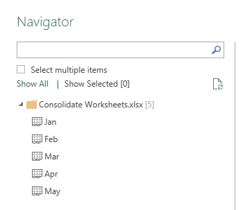
I selected Jan above and then edited the query.  In this sample data, there are no transformations required.  If you need to reshape your data, then now is the time to do it, before you move on.

After you have completed your transformations, you will want to give the query a new name.  The generally accepted approach I have seen is to give the query a prefix like “fn” – I normally call mine fnCombine or something like that.

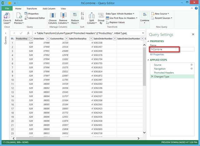
The next step is to change the Power Query Language so it turns this specific query into a function that is generic and can be reused.  There are easy ways and hard ways to do this – I now know the easy way – read on. 

Convert to Function

Switch to the Advanced Editor (View\Advanced Editor) and you will see the Power Query Language code generated by the UI.

Now I have seen more complex versions of the next step, but this is the easy way.  I learnt this when I attended Miguel Llopis’ Power Query session at PASS BA Conference this year.  The thing is you don’t need to write additional ‘let’ and ‘in’ statements as I have seen others do (and as I have done in the past).  All you need to do is to add a line of code that accepts the parameters.

(Parameter1,Parameter2,ParameterN) =>

That’s it.  It is really simple.  So you can see the extra line of code added as line 1 below.  Don’t worry about the other lines of  code from line 5 on.  These were all generated by the UI and are not important for the purpose of this post – yours will be different anyway.  The only lines that matter are line 1 and line 4.  For this demo, just ignore all the others.
(mySheet)=> let Source = Excel.Workbook(File.Contents("C:\Users\matt\Documents\Blogs\Consolidate Worksheets.xlsx"), null, true), Jan_Sheet = Source{[Item="Jan",Kind="Sheet"]}[Data], #"Promoted Headers" = Table.PromoteHeaders(Jan_Sheet), #"Changed Type" = Table.TransformColumnTypes(#"Promoted Headers",{{"ProductKey", Int64.Type}, {"OrderDate", Int64.Type}, {"CustomerKey", Int64.Type}, {"SalesTerritoryKey", Int64.Type}, {"SalesOrderNumber", type text}, {"SalesOrderLineNumber", Int64.Type}, {"OrderQuantity", Int64.Type}, {"UnitPrice", type number}, {"ExtendedAmount", type number}, {"UnitPriceDiscountPct", Int64.Type}, {"DiscountAmount", Int64.Type}, {"ProductStandardCost", type number}, {"TotalProductCost", type number}, {"SalesAmount", type number}, {"TaxAmt", type number}, {"Freight", type number}, {"RegionMonthID", type text}}) in #"Changed Type"

If I just save it now – no other changes – it is now a function.

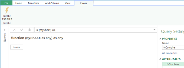
But I’m not finished.  The above function doesn’t do anything, because the parameter that is passed to the function in the first line of code is not used in the Power Query Language anywhere yet.  So I then changed line 4 like this.

Jan_Sheet = Source{[Item=mySheet,Kind=”Sheet”]}[Data],

All I did was replace the hard coded sheet name “Jan” with the Parameter passed to the function in the first line.  So as you can imagine, it is now possible to reuse this function over and over again.  Instead of it being a hard coded single purpose function that operates on the sheet “Jan”, I can now pass any number of different sheet names to the function, and the function will perform the exact same transformation over the specified sheet(s).

Now here is a second tip.  Rather than just changing the required line(s) of code, I recommend you duplicate the line(s), comment out the original line(s) and then change the duplicate copy.  I started to do this because sometimes I needed to come back and make changes to the query after I had converted it to a function.  It is much easier to make changes using the UI, but that is only possible if you convert it back from a function to a normal query.  If you are not an expert in the Power Query Language, it can be very difficult to work out how to “undo” the function conversion.  So if you keep the original line of code, it is much easier to go back to where you started.

After I duplicated the original line of code, what I actually end up with is this (note the double slash to comment out the original line of code – line 4.  And notice the duplicate line of code (line 5) with the modification that accepts the parameter from the function.  As a side bonus of doing it this way, it is much easier to see what changes you have made to the query.
(mySheet)=> let Source = Excel.Workbook(File.Contents("C:\Users\matt\Documents\Blogs\Consolidate Worksheets.xlsx"), null, true), //Jan_Sheet = Source{[Item="Jan",Kind="Sheet"]}[Data], Jan_Sheet = Source{[Item=mySheet,Kind="Sheet"]}[Data], #"Promoted Headers" = Table.PromoteHeaders(Jan_Sheet), #"Changed Type" = Table.TransformColumnTypes(#"Promoted Headers",{{"ProductKey", Int64.Type}, {"OrderDate", Int64.Type}, {"CustomerKey", Int64.Type}, {"SalesTerritoryKey", Int64.Type}, {"SalesOrderNumber", type text}, {"SalesOrderLineNumber", Int64.Type}, {"OrderQuantity", Int64.Type}, {"UnitPrice", type number}, {"ExtendedAmount", type number}, {"UnitPriceDiscountPct", Int64.Type}, {"DiscountAmount", Int64.Type}, {"ProductStandardCost", type number}, {"TotalProductCost", type number}, {"SalesAmount", type number}, {"TaxAmt", type number}, {"Freight", type number}, {"RegionMonthID", type text}}) in #"Changed Type"

If at any time I need to edit the query, I can simply do the following.

1. Put a double slash in front of line 1        //(mySheet)=>
2. Remove the double slash from line 4
3. Put a double slash in front of line 5

And bingo, I am back in business and I can use the UI again.

Save the function again and close.

Create a second query.

Next I created a second query that points to the same file, but this time instead of selecting one of the worksheets I selected the workbook itself.

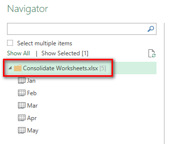
When you edit this folder (which is actually the workbook) you will see a list of all of the sheets in a Power Query window.

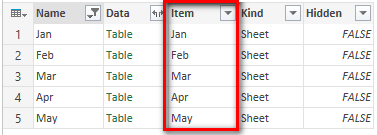
You may have to do some filtering here before proceeding.  In this demo, I filtered out Sheet1 and Sheet2 using the filter icons.  I used the option to filter out rows that begin with the word “Sheet” to make it “future proof”.

So now I have a nice clean list of sheets that are in the workbook, and the name of each sheet is in a single column.  This is the secret sauce.  Because the sheet names are in a column, they can be “passed” to the function – and then the function will process the sheets one at a time.

---

Interested in Learning How to Do this Kind of Thing?

Our New Online Power Query Course just launched this year. You’ll learn Power Query from the best in the business, two Excel MVPs Ken Puls and Miguel Escobar. We’ve included 7 Hours of Self-Paced Video over 31 Courses, with lots of example files, and a Digital Badge powered by Acclaim.

CLICK HERE to claim your spot.

---

Add a custom column to call the function

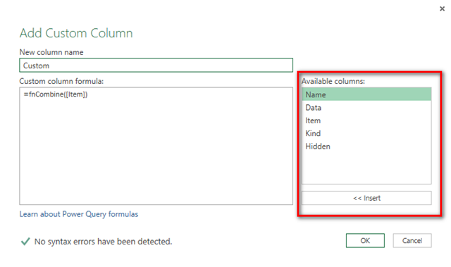
So then I added a custom column – I just typed a hand written formula in the box that calls the function.

Remember I renamed the query to be “fnCombine” – so that is now the name of the function I have to call.  So all I had to do is just write the code using the UI to help me.

=fnCombine([Item])

Power Query is case sensitive, so you have to type it exactly as the name of your function – FNCombine will not work!  Note how I have inserted the [Item] inside the function. [Item] is the column from the earlier step that contains all the sheet names.  All of the column names that exist in the query are conveniently located and available inside the “add column” editing window.

After inserting the custom column, you will see each row of the new column is a full table in its own right.  Each table is the full data from each sheet with the transformations applied.

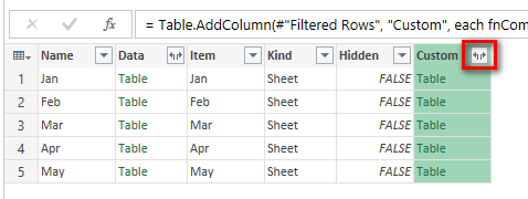
Expand the Column

Now expand the column using the icon shown above.

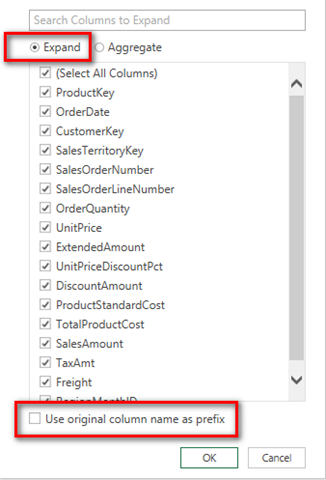
Select the expand option and deselect “use original column name as prefix” down the bottom, then click OK.

Finally remove the first 5 columns that are not needed and you are done.  Close and load as required.

Here is the sample data I used to import.  Feel free to use it to practice.  Sample Workbook

Matt Allington is a professional Self Service BI consultant and Author specialising in Power Pivot and increasingly Power Query based in Sydney Australia.