Dynamic TopN Reports via Slicers, Part 2

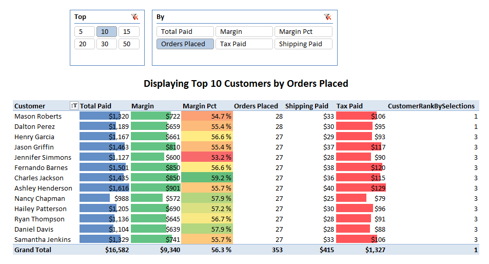
OK, picking up from Tuesday’s post, with the goal of explaining the techniques.

And remember, you can download the workbook here!

Two Disconnected Slicers

Ah, another favorite technique.  Slicer tables that are only intended to populate slicers, never to be related to other tables!

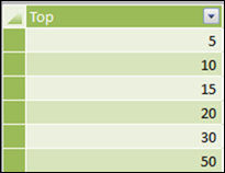
To create these slicers, I literally just created them manually in Excel, then copy/pasted them into PowerPivot:

Behind the Scenes Measures – Harvesting Selections from Slicers

I next write measures that “harvest” the user’s selections from those slicers, just like in the sort by slicers trick:

[Selected TopN Measure] = MIN(MeasureForTopN[ID])

[SelectedTopNNumber] = MIN(TopN[Top])

I use MIN to break ties in case the user is silly and selects more than one value on a slicer.  I could just as easily use MAX, or do an IF(COUNTROWSVALUES()) test, catch the case where more than one is selected, and specify a default value.  (There’s also a new function in V2, HASONEVALUE, that I have not used yet).

Then I write a branching measure – a measure that “becomes” different measures based on conditional tests.  (See the sort by slicers post for more explanation).  In the sort by slicers post I used a nested IF, but now we have SWITCH, and OMG, is SWITCH better:

[Selected TopN Value] =
SWITCH([Selected TopN Measure],
       1, [Total Paid],
       2, [Margin],
       3, [Margin Pct],
       4, [Orders Placed],
       5, [Tax Paid],
       6, [Shipping Paid]
)

Oh PowerPivot team, thank you thank you thank you thank you thank you!   I think I have some mild form of dyslexia that has always made nested IF’s difficult for me to write.  People are always looking over my shoulder saying “yeah, you missed that third closed parenthesis on the second line of the formula” and I stare at them in disbelief.  No more!  I have SWITCH!

OK, so now we have a measure that returns the [Total Paid] amount if the user selects “Total Paid” on the slicer.  Cool.

The Rank Measure, My First Use of RANKX()

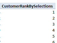
OK, now we need the measure that ranks each customer according to the selected measure:

Here’s the formula:

[CustomerRankBySelections] =
RANKX(ALL(Customer[FullName]), [Selected TopN Value], ,0)

My observations on RANKX:

1. First off, it’s amazing to have it.  Even better than SWITCH – All you have to do is go read my series of posts on writing a rank measure in V1 and you will be sold on RANKX.  It’s way easier to write, and it appears to be much faster to evaluate than the old way.  So let’s not look a gift horse in the mouth.  OK, I’m going to do it anyway.
2. Why do I have to specify ALL() in the first param?  I struggled here, I was just reading the function text for RANKX and all it said for that first param was “Table.”  So I was throwing VALUES(Customer[FullName]) in there, and every customer was coming back ranked as 1.  This is the right function design if flexibility is your overwhelming design goal.  But for the 99% case this is incredibly counterintuitive – for the Excel crowd it would be much better to have a simpler function where all I need to do is specify a column – no ALL(), no VALUES(), just a “raw” column.
3. That third param – I still have no idea what that third param means.  You can leave it blank though and it doesn’t cause any harm.  So um, leave it blank.
4. Fourth param – set to 0 when you want the largest number to be ranked 1.  If you omit this parameter, it defaults to the other way, which is backwards IMO for a function named RANK.  (The best team in the NFL each year – is their rank 1 or 32?)

(Microsoft folks, please think of this as input on the future, friendlier RANK function you give us, and not sour grapes.  I’m super happy to have the function, but the friendlier you can make it, the better).

The “Should Customer Be Included?” Measure

At this point, if we were always just doing Top 10, and not a slicer-controlled Top N, we’d be done.  We’d just set a filter on the pivot to always show top 10 customers by [CustomerRankBySelections] and everything would be great (in fact we could have skipped [CustomerRankBySelections] altogether and just done a top 10 filter by [Selected TopN Value], the branching measure itself.

But we need one more simple measure:

[Should Customer Be Included] =
IF([CustomerRankBySelections]<=[SelectedTopNNumber],1,0)

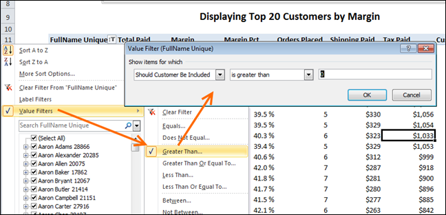
Then we filter the pivot to only show rows where that measure is > 0 (or = 1)

Make Sure Customer Names Are Unique!

As pointed out in the comments on Tuesday’s post, my original FullName column was not unique – there is more than one customer named Willie Xu for instance, and this approach combines them into one “super customer” who unfairly sneaked into the top 10.

So you can either create a unique customer name and use that on your pivot:

Or in theory you can change your RANKX measure to use the behind the scenes unique ID instead.

I have had NO succcess with that yet however.  When I use ALL(), like I did in the original measure, it becomes so slow that the pivot never finished calculating, I end up canceling it.  And when I use VALUES() instead, every customer comes back ranked as 1.

This Formula Never Finished Running:

[CustomerRankBySelections] =
RANKX(ALL(Customer[CustomerKey]), [Selected TopN Value], ,0)

And this formula ranks all customers as 1:

[CustomerRankBySelections] =
RANKX(VALUES(Customer[CustomerKey]), [Selected TopN Value], ,0)

So let’s call this a work in progress.

The Readout

As an extra touch of class and usability, we often like to do something like this:

That readout is just a merged cell with a formula in it:

The two cells referenced in that formula are interesting.  One is a cube formula:

Here’s the formula in text:

=CUBEVALUE("PowerPivot Data", "[Measures].[SelectedTopNNumber]",Slicer_Top)

Note how that formula is parameterized by the name of a slicer?  That allows the formula to be sliced by the slicer, just like a pivot.

The other cell is the top cell on rows in a pivot:

That pivot has a slicer connection established to the same measure-selector slicer, and also has the same field on rows as the slicer field itself.

I could have used a cube formula for this part as well, but that would have required me to write a text measure, and I was feeling lazy 🙂

For more on this stuff see the Cube Formulas category, as well as a series of posts on getting and using slicer values in formulas.