Profit & Loss (Part 2)–Compare and Analyse

Guest post by David Churchward

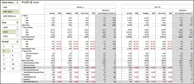
In my recent post, Profit & Loss-The Art of the Cascading Subtotals, I went through a basic P&L layout with some relatively complex DAX measures to display and hide row headings as appropriate together with calculating accurate values.  In order to make this report more meaningful, it needs comparatives and further analysis.  In this post, I’ll build on the P&L created in part 1 to create some of the key elements of the layout shown above including Actual values, Budget values and Prior Year values for a selected period and the associated year to date (YTD).  In part 3, I’ll go on to show how the percentage calculations work and maybe some pointers for making it look REALLY good!

Time Intelligence

As our report is considering different timeframes, we need to establish a time dimension and condition slicers to select a required timeframe.  From this, we can determine the required time parameters for use in subsequent measures.

We need to establish 4 tables that we will use for time intelligence.  These are fully explained in my recent post Slicers for Selecting Last “X” Periods.

Dates – this is a list of sequential dates covering the timespan of our dataset.  This is linked to a date field in the dataset.

Year – this is a sequential list of years covering the timespan of the dataset.  This table should NOT be linked to the core dataset (or fact table if you prefer).

Period – this is a sequential list of periods, normally from 1 to 12 where a period is a calendar or fiscal month.  Again, this table should NOT be linked to the core dataset.

Year_Period – this is a list of year and period combinations covering the timeframe of the dataset.  This table also carries other relevant dates and attributes that relate to the date records contained within.

Year_Period is linked to both Year and Period on a many to one basis.

Creating Time Parameters

I create time parameter measures on the Year_Period table.  We need the following time parameters for use in our measures:

Selected Month End Date – this tells us the date relating to the end of the month for the selected period and year combination selected by the user on slicers.  Month end dates don’t change and so I’ve been able to hold this as a field in the Year_Period table which means that I just need to capture the associated value and deal with the fact that multiple selections could be made (or no selection at all).  This is done using:

Selected_Month_End_Date = LASTDATE(Year_Period[Month_End_Date])

It should be noted that I’m always using the LASTDATE function in these measures.  This is to ensure that I always evaluate to one result.

Selected Month Start Date – again, this is available in the Year_Period table as the value doesn’t change for any selected date

Selected_Month_Start_Date = LASTDATE(Year_Period[Month_Start_Date])

Selected Prior Year Month End Date – once again, we could make this available on the Year_Period table as the value won’t change and, for efficiency reasons, I would tend to do that.  However, for the benefit of showing an additional method, I’ve chosen to use the DATEADD function here.

Selected_PY_Month_End_Date = LASTDATE(DATEADD(Year_Period[Month_End_Date],-1,YEAR))

DATEADD requires the syntax DATEADD(dates, number of intervals, interval).  The dates element is a table / column expression which details which column to use in the evaluation.  I use –1 as an interval to go back in time (essentially turning DATEADD into DATEMINUS which of course doesn’t exist as a function!).  The interval is the timeframe type by which you wish to adjust and this can be DAY, MONTH or YEAR as my date field doesn’t contain any time elements.

Selected Prior Year Month Start Date – let’s not let this drag out and get boring!  Measure below:

Selected_PY_Month_Start_Date = LASTDATE(DATEADD(Year_Period[Month_Start_Date],-1,YEAR))

Selected Year Start Date – DATEADD is used again here but we need to know how many months to go back.  As the user is selecting a period and year combination, we can pick up the period that is being evaluated from the slicer and use this to work back to the first date in the year.

Selected_Year_Start_Date = LASTDATE(DATEADD(Year_Period[Next_Month_Start_Date],MAX(Year_Period[Fiscal_Period])*-1,MONTH))

As I’m using Fiscal Periods (in the main I use July as Period 1), I need to pick up the selected Fiscal Period (ensuring that I evaluate to one answer – hence the MAX function) and then multiply by –1 to work backwards through time as opposed to forwards.

Selected Prior Year Start Date – this is getting boring Churchy – move on:

Selected_PY_Year_Start_Date = LASTDATE(DATEADD(DATEADD(Year_Period[Next_Month_Start_Date],MAX(Year_Period[Fiscal_Period])*-1,MONTH),-1,YEAR))

Nothing tricky here.  I just take one year away from Selected_Year_Start_Date.  I’ve used a nested DATEADD to show how it’s done as opposed to using the answer from Selected_Year_Start_Date.  There’s multiple ways of doing these things!

With that done, I think we’re finished with date parameters.  Let’s get on with putting them to good use.

Applying Time Intelligence to my Cascade_Value_All Measure

You may recall in Profit & Loss-The Art of the Cascading Subtotals that the key outcome was a measure called Cascade_Value_All.  We can now start dissecting this measure by overlaying time intelligence and filters to capture the values that we need on our report and this is all done safe in the knowledge that Cascade_Value_All will manfully ensure that report headings behave appropriately.

I’ll construct these measures in sections to make them clear.  You can ultimately combine these into fewer measures if required.  Let’s start by overlaying time intelligence.  This is done using the DATESBETWEEN function.  I tend to use this regularly as I’ve never encountered a situation where I’m working with calendar years!

We need 4 measures – current month, current month last year, current month YTD, current month YTD last year.

Cascade_Month =

CALCULATE(

[Cascade_Value_All],

DATESBETWEEN(

Dates[Date],

Year_Period[Selected_Month_Start_Date],

Year_Period[Selected_Month_End_Date]

         )

  )

In this measure, we’re essentially filtering the outcome of Cascade_Value_All down to the underlying transactions that fit between the start and end dates provided to the measure.  This means that our other 3 required measures that represent current month last year, current month YTD and current month YTD last year are exactly the same although the start_date and end_date elements highlighted in bold are substituted with the relevant date parameters calculated in the Creating Time Parameters section above.  Let’s call these three measures Cascade_Month_PY, Cascade_YTD and Cascade_YTD_PY.  Don’t worry as all measures will be available in the workbook that I’ll make available with Part 3.

Filter Actual and Budget

In our P&L report, we have two types of data being Actual and Budget.  These are all records in the main fact table dataset and each record is denoted with a Data_Type field (value of 1 denoting Actual and a value of 2 denoting Budget).  This field is linked to a DIM_DataType table.

To filter the dataset for the current month measure (I won’t go through them all as I’m sure you’ll get the idea), I use the following measure:

Cascade_Month_Actual =

CALCULATE(

[Cascade_Month],

DIM_DataType[Data_Type_Name]=”Actual“

      )

This will give us the correct values for the selected month representing the “Actual” dataset.  We can create an equivalent for “Budget” simply by changing the filter value.

I create a “Prior Year” version of Cascade_Month_Actual by substituting [Cascade_Month] with [Cascade_Month_PY], ensuring that our filter is set to “Actual”.

Why Filter “Actual” and “Budget” instead of simply adding them to the Column Headings in the Pivot Table? – Use of Static Columns

I could avoid multiple measures by simply using my [Cascade_Month] measure (together with the other time adjusted measures) and adding Data_Type as a column heading.  There’s a few reasons why I wouldn’t do this in this particular case.  That’s not to say that it isn’t a valid approach in the majority of other examples.  My reasons are:

1. I want to ensure that my columns remain static.  If, for whatever reason, I evaluate to not having a budget for a particular slice of the data, I don’t want the column to disappear.
2. OK, so number 1 might be a bit weak!  I’m also aware that the budget for Prior Year probably isn’t relevant so I don’t want to see it.  My prior year comparison is being used to evaluate my current year actual.  I don’t want prior year budget getting in the way so I only want to see actual for my prior year dataset.
3. I want to add a blank column between my “Month” information and my “YTD” information.  Again, a bit weak, but buy-in from users is partly about how pretty is looks and I think it looks prettier this way.
4. If I use a field on my column headings, I could get multiple rows dedicated to my column titles.  As a taster to what’s coming up, I don’t want to use the Pivot Table headings because they’re ugly on this report.  I’m going to create my own damn it!  If I use static columns, I can guarantee only one heading row which means I can hide it and create my own prettier version!
5. This is probably the most compelling reason!  It’s quite normal for Budgets to be superseded by Revised Forecasts.  With static columns, I can ultimately provide a slicer that allows the user to select whether they want to see budget or revised forecast information against actuals.

Note – there’s always a balance to be considered when making an assessment like this.  On the one hand, this may “look pretty” and avoid displaying information I don’t want but if performance suffers than you’re onto a rough deal!  With these measures, I haven’t had a performance issue with quite large datasets so I don’t have to compromise appearance just yet but there’s no doubt that it’s less optimised than constructing one measure and adding a field to column headings.

When We Pull This All Together……

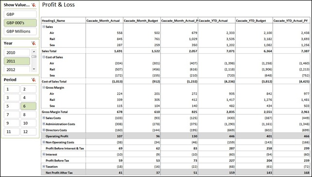
I add the six new measures to the P&L report and attach slicers for Period [Period] and Year [Year], tidy up a bit and produce the following:

Look out for Part 3 when we’ll add ROS (Return on Sales) percentages and variance calculations whilst also having a tidy up of the layout.