Complex Customer Cohort Retention Using PRODUCTX

Post by Rob Collie

First, a Few Quick Updates…

1) Just a reminder that enrollments are open for the live, in-person two-day classes taught by me (Rob) in Indianapolis and Washington DC (in October and November, respectively.)  Sign up now – those dates will be upon us sooner than we all realize!

2) The pre-order for DAX 2nd Edition is going Great!  Thanks to everyone who has pre-ordered and/or contributed.  PRE ORDER  if you have not already, and don’t forget the exclusive swag rewards like the sticker, poster, and t-shirt.

3) Ola Freaking Rosling is now using Power BI, and threw us a “shout-out!”  OMG, check out this tweet.  I nearly peed myself:

If you don’t recognize the name, his dad is Hans Rosling, the speaker in the first TED talk I ever watched:

Click Image to View the Talk

…In which he did the animated bubble chart demo that I’m 100% positive was the inspiration for Amir Netz adding animated bubble charts in the next two product releases

Here’s Ola and Hans co-presenting on the state of world health and social justice, via data of course:

Again, Click to View the Talk

A celebrity in that Google-y, Apple-y, Silicon Valley-y “doing good with data in the public interest” space using Power BI and saying that Power BI is awesome, and that he’d previously been scared off by all the anti-MS propaganda…  well that is simply awesome.

But I won’t lie – that he gave US a mention in that tweet – I *do* find that to be even cooler.  I’m human.  I can’t help it.  I smile every time I think about it.

Slaying the “White Whale” of Variable-Rate Forecasting with PRODUCTX

“Arrrrr!  We Be Meeting Again!”

OK OK…  time to circle back to one of my only “defeats” EVER, and settle the score!  Yes, this problem…  well it beat me up pretty badly about 18 months ago.  I eventually solved it, but not in a way where the formula was even remotely explainable or maintainable.

I’ve done some posts about exponential growth forecasting before.  In both of those posts, I used the POWER() function to multiply out the increasing or decreasing series.  (10 percent growth each year, for five years translates to 1.10 raised to the 5th power).

But both of those posts assume the growth factor is STATIC.  Meaning, if you forecast 10 percent growth per period, it’s 10 percent growth for EVERY period.  That nice, steady percentage allows us to use the POWER function to handle all the multiplication.

Those were easy mode, in other words.  But then, later, I wrote another post that handled variable rates.  I leaned heavily on Jeffrey Wang from Microsoft for that one, because DAX didn’t have a PRODUCTX function at the time.  That was some complex mathmagic-land stuff – converting a multiplication series into a sum by using logarithms and exponents, but it got the job done.

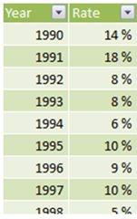
This was harder:  Each year had its own specified growth rate.
(But STILL…  that rate applied to EVERYONE for that year – my next example is worse)

Still, though, even THAT was easy mode compared to the problem I encountered a year later!

What if your growth rates are still variable, but you have multiple populations of customers moving through the forecast, and as those populations “age,” we must look up their growth rate based on how long ago we acquired them?  Meaning, for a given calendar year’s forecast, each group of customers (grouped by their “age”) has to be treated a bit differently?

Here, it’s probably easier to show you:

The Left Hand Column is No Longer a Calendar Year – It’s a Customer’s “Age!”
(Oh, what’s that you say?  That table looks funny?  It’s Power Pivot in Excel 2016!)

In short, THIS problem was a farkin disaster.  The crazy “logarithms, exponents, and SUMX” workaround to create our own version of PRODUCTX was hard enough on its own, but when I THEN had to “nest” THAT contraption of a formula inside ANOTHER crazy series of loops, well, it would have given Obi-Wan one of those terrible disturbances in the Force.  It was an unsatisfactory result.

Now We Have PRODUCTX, for Realz!

With Excel 2016 and Power BI Desktop, though, we now DO have a real PRODUCTX function, so that “inner” complexity is removed.  At least in theory.  So I’ve been meaning to circle back around and give it a shot.

In short…  I beat this sucker.  It was still a bit chewy, but seriously, 20x easier than the last time I tried it (without benefit of PRODUCTX).

Here’s the model:

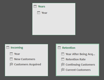
Three Tables, No Relationships.

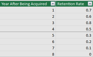
The Three Tables:  Intentionally Small, But this Technique Will Work With “Bigger” Data

Description of the Problem

Let’s describe the problem in English, using the tables above as a reference:

1. Each year from 2008 through 2015, we have a “known” number of new customers who “walked in the door.”
2. We also have research that tells us that one year after we acquire a customer, there’s a 70% chance that customer is still around.
3. Any customer who “survives” that first year then has a 60% chance of sticking around for the following year.
4. We actually get a “bump” in customer loyalty in year three – if you’ve stuck with us that long, chances are good that you REALLY like us, and we’ve found we retain 80% of such customers for the next year.  (Of course, that’s 80% of 60% of 70% of the original incoming customers, so it’s still a minority in the bigger picture).
5. But then, customers tend to become “satisfied” or “weary.”  For whatever reason, customer retention falls off after that, and in year 4 we only keep 50%, followed by 30%, 20%, 10%, and ultimately 0%.
6. So, if we want to project how many customers we’re going to have “in the system” for year 2019, we have a very complex problem.  Each of the 2008-2015 populations must be “aged” differently, and then all of those results must be blended together into a unified projection.  Yikes.

Diagram of the Problem

If we want to forecast total customers for 2016, it would look like this:

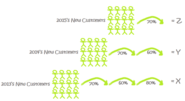
If We Add X + Y + Z, We Get Our Answer
(There are actually other populations involved, too, Like 2012 and 2011, But The Diagram Was Getting Too Big.  So it would actually be more like U + V + W + X + Y + Z, but you get the idea.)

OK, Enough Setup.  Here’s the Resulting Pivot.

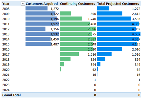
See?  Done.  That Last Column is the Final Measure.

The Formulas

From right to left in the pivot above:

Total Projected Customers:=
[Continuing Customers]+[Customers Acquired]

Customers Acquired:=
CALCULATE(SUM(Incoming[New Customers]),
FILTER(Incoming, Incoming[Year]=MAX(Years[Year])))

Continuing Customers:=
SUMX(FILTER(Incoming, Incoming[Year]<MAX(Years[Year])),
PRODUCTX(FILTER(Retention,
Retention[Year After Being Acquired] <=
MAX(Years[Year])-Incoming[Year]
),
Retention[Retention Rate]
)
*Incoming[New Customers])

OK, so that third formula was the hard one.  But WAY easier than before, when we didn’t have PRODUCTX!

Oh???  You want me to EXPLAIN it???  Sheesh folks, it’s 1 am here and I’m catching a taxi at 6:30 am.  I’m gonna be a zombie tomorrow as I fly from one side of the country to the other.

Seriously, I’m just gonna have to take a rain check for tonight. Maybe I’ll explain, tomorrow, in the comments