Nested SUMX or DAX Query?

by Matt Allington

I was helping a friend out recently with an interesting problem.  It all started with a SUM( ) that wasn’t behaving. It quickly became a SUMX( ) problem but evolved into a DAX Studio/Query problem.   Let me explain.

The Root Problem – Same Store Sales

Many retail businesses open and close stores throughout any given year.  This creates a problem because it is difficult to determine if business growth is vertical (increased sales within existing stores) or horizontal (expansion of the store base).  It is common to do analysis on “same store sales” where you only include stores that had sales for the entire period this year and also last year. There are quite a few posts already on this topic on p3adaptive.com, but this is a good opportunity for me to talk about SUMX and also DAX as a query language.  I have reconstructed the scenario with some test data.  You can download the workbook here if you want to take a look.

I started off with some base measures as follows:

A. Total Sales:=SUM(Sales[Extended Amount])

B. Total Sales LY:=CALCULATE([Total Sales], SAMEPERIODLASTYEAR(Calendar[Date]))

There are a few different ways to work out sales last year, but I have used SAMEPERIODLASTYEAR above and this works just fine in this instance.

When placed in a Pivot Table, these measures look like this.  I only want to analyse sales where there is a value for This Year (TY) AND Last Year (LY) for each particular store, and this table makes it easy to visualise when that occurs.

Pivot Table 1

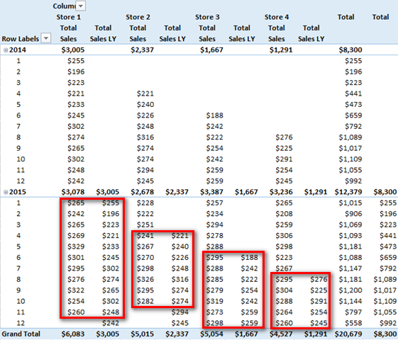
Notice how my test data is set up so there are some stores opening and closing at different times of the year in 2014 and 2015. Creating good test data and setting up a pivot table that reflects what will happen in real life is essential if you want to eliminate rework and get the DAX right the first time.

Let’s start with a simplistic Same Store Sales solution that only works in some circumstances.

C. Same Store Sales TY Simplistic:=CALCULATE([Total Sales], FILTER(Stores, [Total Sales] > 0 && [Total Sales LY] > 0 ) )

D. Same Store Sales LY Simplistic:=CALCULATE([Total Sales LY], FILTER(Stores, [Total Sales] > 0 && [Total Sales LY]> 0 ) )

Both of these above simplistic Same Store formulae will work in very limited scenarios where the Pivot Table provides an initial filter context for the time period.  Note in Pivot Table 2 below how “Same Store Sales TY Simplistic” is showing the correct values for each month in 2015 (shown as 1 in the Pivot below).  If you look Pivot Table 1 above and compare it with Pivot Table 2 below, you can see Store 2 opened in month 4 2014 and closed in month 10 2015, so Same Store sales in any given month (shown in box 1 below) are all correct.

Pivot Table 2

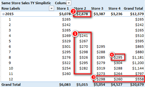
The problem is that the 2015 total (shown as 2 above) is not correct.  The sub total for Store 2 2015 is showing the value $2,678 but if you add up all the values in the box 1 above, the numbers only add up to $1,977.  This is a common problem that can normally be solved by using SUMX.  (Note: there are lots of other posts about SUMX at p3adaptive.com if you are interested).  This “doesn’t add up” problem is not occurring in the Grand Total for rows (shown as 3 above) because the FILTER function in my DAX formula is iterating across the Stores table and hence each store is being treated as an independent entity for FILTER evaluation purposes.  The cause of the problem (shown as 2 not adding up correctly) can be a little hard to understand unless you truly understand how Power Pivot works under the hood.

How the Power Pivot Engine Works.

Power Pivot first of all takes the initial filter context from the Pivot Table and filters the underlying tables so that only the relevant rows are presented to the formula engine.  Let’s take the cell highlighted as 4 above.  The initial filter context from the Pivot Table has filters on Stores[Store]=”Store 4”, Calendar[Year]=2015 and Calendar[Month]=8.  So the only rows in my sales table that are available to the pivot table for the calculation of this cell are the rows that match this filter context.  Once the underlying tables are filtered to reflect this filter context, then and only then does the formula engine kick in and calculate the answer to my DAX expression:C. Same Store Sales TY Simplistic:=CALCULATE([Total Sales], FILTER(Stores, [Total Sales] >0 && [Total Sales LY] >0 ) )

Given that the cell shown as 4 above is filtered for the month of August 2015, the part of the formula [Total Sales] > 0 && [Total Sales LY] > 0 will successfully work out if the current month needs to be included.  If there are sales for “this month, this year” and also the “same month last year” for this store, then the sales for TY will be included and returned to this cell in the Pivot Table.  But the problem with the sub total row (shown as 2 above) is that there is no such filtering on months.  So the initial filter context coming from this sub total in the above Pivot Table is simply Stores[Store]=”Store 2” and Calendar[Year]=  2015.  There is no filter on month.  So when the part of the formula [Total Sales] > 0 && [Total Sales LY] > 0 is evaluated, it is evaluated across the entire year instead of a single month.  As long as there was a single sale in the year 2015 and also a single sale in the year 2014 for an individual store, the entire year’s sales for that store will be included in the sub total (shown 2 above).  You can see this total $2,678 in Pivot Table 1 – it is the total for all month sales for Store 2 (you can check it against the total shown in Pivot Table 1 to confirm).

So in short, the initial filter context coming from the rows in the Pivot Table is ensuring the Same Stores sales by month is working at the row level.  As soon as you remove the initial filter context on month by removing the months from the Pivot Table (or like is happening at the sub total level), this formula is not going to work.  Whenever this problem happens, my first instinct is to jump to SUMX.  SUMX is an iterator and hence SUMX can simulate the existence of rows in a Pivot Table.  Take the following formula.E. Simple SUMX:= SUMX(Calendar, IF( [Total Sales]  > 0 && [Total Sales LY] >0,[Total Sales] ) )

Now this formula (E) iterates over the Calendar table and checks to see if there are sales this year as well as last year (at a day level of granularity because my Calendar table has day level data).  If there are sales in both years, then the sales are included in the resulting total.  But this creates a new problem that didn’t exist in formula D.  The new problem is there is no longer an iterator working on the Stores table.  Without the FILTER( ) on the Stores table (or maybe another SUMX), the totals for All Stores will not add up correctly.    In fact the same problem that occurred with “Months” will now occur with “Stores”.  When the formula is at the sub total level, the sales for all stores will be included in the result.

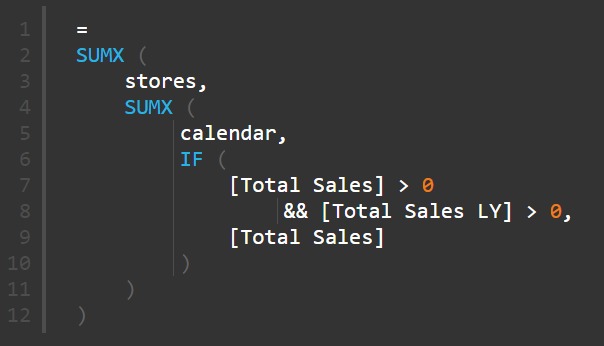
So one way to solve this problem is to use a double iterator and iterate over both the Stores table and also the Calendar table.  You can do it like this with a double SUMX

F: Double Nested SUMX

..or a FILTER with SUMX.

G: FILTER and a single SUMX.

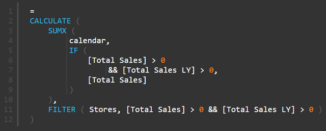
But either way, this is not going to be very performant because they both have double iterators.  So I asked around and Scott from TinyLizard.com suggested I check out SUMMARIZE.  I have watched Alberto Ferrari’s Many to Many presentation often enough to know that SUMMARIZE was a likely contender.  I can still hear Alberto saying ‘SUMMARIZE uses a single Vertipaq operation…’ and hence I know SUMMARIZE is going to be faster than using a double nested SUMX pattern.

My journey to find the right DAX Query formula.

Anytime I start using DAX as a query language to solve a particular problem, I ALWAYS fire up DAX Studio.  It is not that hard to use and it allows you to “see” the results of your formulae as you are writing them.  I always write my exploratory DAX formulae from the inside out, building it up one piece at a time, and DAX Studio makes this process a snap.   I did a quick refresher on SUMMARIZE at SQLBI.COM and I started out with this:

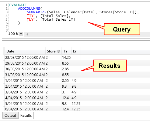
SUMMARIZE is a bit like GROUP BY in SQL and it creates the first 2 columns of the table in the image above summarised to the level specified.

If you read the article at the above SQLBI.COM link the clear advice is to use ADDCOLUMNS rather than SUMMARIZE when creating new columns of data on the fly, so that is what I did above.  Once I executed this query (shown in the image above) I could ‘see’ that this was giving me what I needed (in the results window above).

The next step was to filter out the columns that didn’t have sales for this year as well as last year.  So I wrapped the above Query inside a FILTER and got the results below

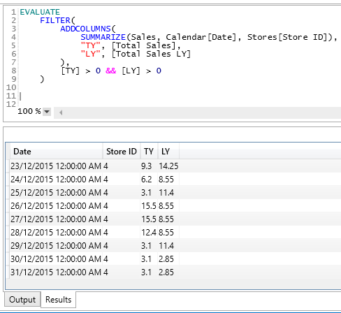
Now that I could “see” that my DAX Query was correctly returning a table of only the values that I needed, I then realised that I could easily swap out Calendar[Date] for another column in my Calendar table.  This has the effect of making this table smaller (and hence presumably faster to execute) while still giving me the level of granularity I needed for my reporting (monthly in this instance).  So I swapped out the [Date] column for the [YYMM] (year/month ID column).  If you were doing Same Store sales by week, then you would need to use a WeekID column here instead.

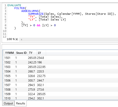
The last step was to wrap this table inside a CALCULATE to get the final result.

H: SUMMARIZE, ADDCOLUMNS and FILTER

I just repeated the process for [Total Sales LY].

Now the reason the above formula works and the original formula (C) doesn’t work is because the above formula is not relying on the initial filter context from the Pivot Table to work.  The SUMMARIZE potion of the query creates a summarised table containing all the possible month-year combinations and the Store ID.  Then the ADDCOLUMNS portion of the formula kicks in.  ADDCOLUMNS has a row context as it works through the SUMMARIZE table, and this row context is converted to a filter context by the implicit CALCULATE function that is part of the [Total Sales] and [Total Sales LY] measures. The new columns TY and LY therefore get populated with the total sales for that store for that month in the row/filter context.  The FILTER portion of the formula then filters out the periods that should not be included (those that don’t have sales in both years).  Because it is operating over the table produced on the fly by this query, it works regardless if the Pivot Table has a filter on Months and/or Stores or not.

So why is the Query approach better?

There are 3 formulae that I have discussed here that all work for Same Store Sales:

• F: Nested SUMX
• G: SUMX with FILTER
• H: SUMMARIZE with ADDCOLUMNS and FILTER

The nested SUMX is going be the slowest to execute.  This formula has a SUMX nested inside a second SUMX.  SUMX is an iterator and hence it will step through every row in the table 1 row at a time.  And given the SUMX are nested, there is a multiplicative effect.  If there are 500 stores and 730 days, then there will be 500 x 730 iterations.  And then there is the filtering and calculation on top of that and remember this is repeated for EVERY CELL in the pivot.

The SUMX and FILTER is a bit better, but FILTER is also an iterator.  The benefit of this second formula is that at least they are not nested.  So FILTER is executed first (730 iterations) and SUMX then kicks in, so there are 500 + 730 iterations.

Finally the SUMMARIZE with ADDCOLUMNS and FILTER is going to be the most performant.  SUMMARIZE leverages the power of the Vertipaq Storage engine to rapidly create a table on the fly.  ADDCOLUMNS quickly creates the required sub totals so that this table is as small as possible but contains all the information required for the calculation.  By the time FILTER is asked to do an iteration, most of the hard work has already been done by the storage engine and hence FILTER only has to work across the smallest possible table of data.  The result is a very efficient and performant calculation.

Matt Allington is the Author of the soon to be released book Learn to Write DAX, and provides Self Service BI Consulting and training in Australia.