The scenario – source data sheets that are structured differently!
Does Power Query sometimes seem too rigid? It’s great for defining a sequence of transformations to clean your data but requires the incoming data to be in a consistent format. Today, I want to talk about a technique for dynamically handling sheets with different structures.
You can download a zip file with the updated sample .pbix and the .xlsx workbook that feeds into it to follow along with here.
Be sure to update the query (the Source step path) to point to your own local machine.
Let’s look at my sample data. Suppose my sales manager sends me a monthly sales report structured similarly to that below:

This table looks pretty clean, right? Using Power Query, you can load this sheet, remove the first two rows and columns, unpivot the data, and you have the numbers you’re looking for in tabular format.
Patting yourself on the back, you file the report away until February rolls around. The Sales Manager sends you the new numbers, and you hit refresh, and… an error! Peeking at the data, you see that he changed the layout of the file and also added new salespeople to the matrix!


As enjoyable as it would be just to tell the manager to stick to a consistent format, sometimes this isn’t realistic or feasible. So, let’s look at how we can use Power Query to handle this chaos:
- Identify the header name for the column that demarcates the beginning of the matrix.
- Automatically detect rows up to that header row.
- Automatically detect columns up to that header column.
- Remove the extra rows and columns, leaving you with a squeaky-clean dataset.
- Unpivot the matrix for each sheet and append into a single dataset.
STEP 1: IDENTIFY THE TARGET HEADER ROW AND COLUMN:
Looking back at our sample data, you can see that there is a common cell in all our sheets that lies at the upper left of the data we want to extract. In this case, the target cell is the “Region” header. We want to remove all rows ABOVE that cell and all columns LEFT of that cell without hard-coding the location of that cell.
STEP 2: LOCATE THE HEADER ROW DYNAMICALLY:
We need some way to identify where the header row starts so that we can remove rows up to that point. This functionality is something that I would have thought is built in by default, but surprisingly is not! Luckily our friend Ken Puls over at ExcelGuru.ca came up with [a solution] for this which I’ve adapted slightly for our purposes.
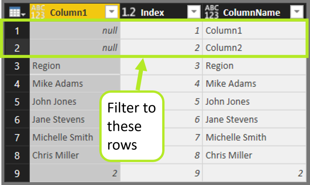
Load your first worksheet into Power Query, add an Index column, and filter the table to the target value from step 1:
- Add Column > Index column > From 0.
- Add a custom step (click the fx button in the formula bar).
- Replace the formula with some custom M code: Table.FindText(#”Starting Table w/Index”, “Region”). Name the step “Filtered to Header Row.”

Note that you’ll want to replace the yellow-highlighted text with the Target Header name from step 1. Table.FindText() scans the entire table for the target text and returns any row with that value. So be careful that your dataset doesn’t have that exact target word in other places!
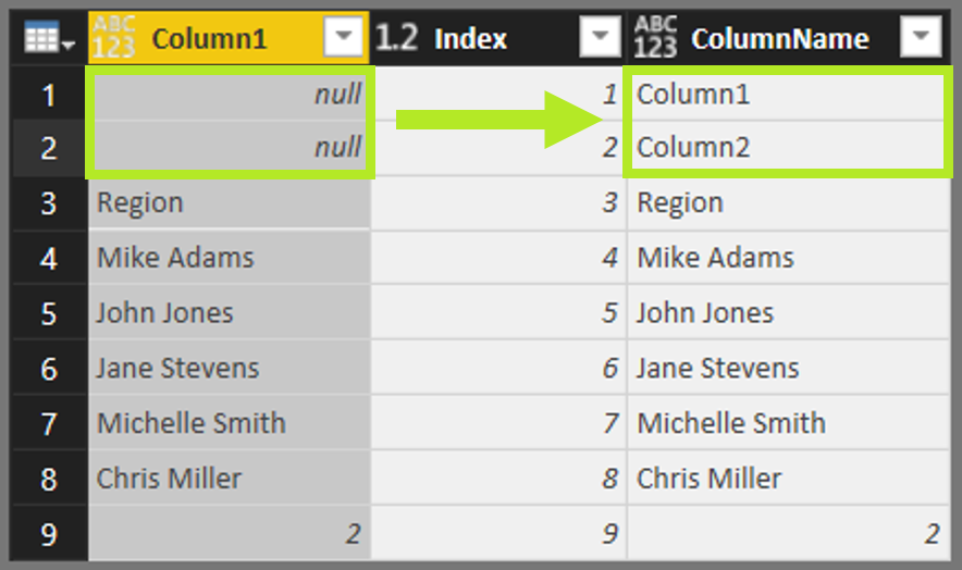
Now we have our header row isolated along with the Index value for that row. Rename the step to “Filtered Header Row” as we’ll come back to this shortly.

STEP 3: DETECT THE COLUMNS TO DELETE
Let’s move on to the more difficult part: dynamically removing leading columns. We have a bunch of columns, and we want to eliminate the first X, up to our target column. We’ll leverage the technique above and add some P3 Adaptive secret sauce.
First, transpose the #”Filtered Header Row” step and add an index. That will make a single row table into a single column table that we use to identify the columns to remove.
- Transform > Transpose.
- Add an index column: Add Column > Index column > From 1.
- To handle blank columns in the header row (always a possibility in dirty data), add a custom column that checks if the column list has any nulls: Add Column > Custom Column > if [Column1] = null then “Column” & Number.ToText([Index]) else [Column1].

Our goal is to delete all columns left of the “Region” column (or above “Region” in the transposed table) so let’s find the index of that row:
- Right Click Column1 > Text Filters > Equals > “Region”.

We’re building upon Ken’s technique of finding the Index that corresponds to a target cell but this time with a transposed table. Since we’ll reference this number a couple of times, let’s Drill Down to just the Index number so that we have an easily referenceable step:
- Right-Click on the Index value > Drill Down.
- Rename that step to “TargetColumnIndex”.
Now, jump around a bit and reference the original column list and filter it down to include ONLY the rows that have an index number less than the target column.
- Click the fx button to insert a New Step.
- Revise the M code to point to the full column list: = Table.SelectRows(#”Added ColumnName”, each [Index] < #”TargetColumnIndex”.
Let’s break down what we’re doing here: the outer Table.SelectRows filters the inner table #” Added ColumnName” down to all rows that have an Index less than the “TargetColumnIndex” value we isolated a couple of steps ago.

Finally, remove the helper columns keeping only “ColumnName,” and you have a nice list of columns to exclude!
STEP 4: REMOVE THE ORIGINAL EXTRA COLUMNS AND ROWS
We now have all the pieces we need to eliminate our junk rows and columns! Let’s jump back to our original query and clean it up.
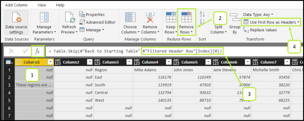
Create a new step and change its code to reference the Starting Table:
- Click fx > rename step to “Back to Starting Table” > change code to = #”Starting Table”.
- Home > “Remove Top Rows.” Enter any value for the parameter.
- Edit the M code directly and change the 2nd parameter of Table.Skip(#”Back to Starting Table,” #”Filtered to Header Row”[Index]{0}), in this case, we want to reference the step where we isolated the header row number from earlier.
- Home > Use First Rows as Headers.

Boom! We’ve dynamically eliminated the top rows!
Now for the final act, we’ll tweak Table.RemoveColumns (when you do “Remove Columns” Power Query uses this function) to use a dynamic parameter! Remember that list of columns we generated earlier, the list we want to extract? That’s what we’ll input into Table.RemoveColumns.
First, select any one of the junk columns and right-click > “Remove Columns.” Take a look at the formula that Power Query generated.
- Table.RemoveColumns(#”Promoted Headers”,{“Column1”}).
We know that Table.RemoveColumns requires a list for its second argument, so we can reference the list of columns to remove from an earlier step:
- Table.ToList(#”Columns to Remove”).

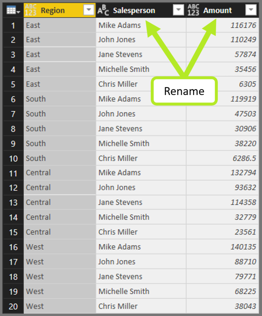
Now we’re left with a clean matrix which we can easily unpivot without any problems.
- Right-click the Region column > Unpivot Other Columns.
- Rename columns something useful.

STEP 5: Convert magic query to function
- The final step is to convert your magic query into a function so that you can apply this dynamic transformation to each file/worksheet that needs to be unpivoted.
To see how the final combined query looks with the function, please download this file here.
Conclusion:
Using the technique of identifying a target row and column, you can create extremely powerful and dynamic queries that can handle input files that aren’t always perfect, because let’s face it, you can’t always rely on training or data validation to prevent end users from modifying your perfect templates. Our job as data modelers is to make the end user experience as friendly as possible by foreseeing and handling exceptions.
If you have any ideas on how you might use this in your reports, please feel free to share in the comments section!
EDIT: Reader Mike Ward posted a very insightful comment on a more elegant way to remove leading rows and columns. His method not only eliminates a few steps in the Query but also allows for the same process to be applied to removing leadings rows as to leading columns. Furthermore, its use of “List.Contains” enforces an exact match on the Target Row/Column identifier. I recommend interested readers review his comment from August 3rd, 2018 and then review the query titled “Jan_MikeWard” in the updated PBIX file (download here).
Thank you for sharing, Mike!
Come for the Techniques, Stay for the Business Value!
We get it: you probably arrived here via Google, and now that you’ve got what you needed, you’re leaving. And we’re TOTALLY cool with that – we love what we do more than enough to keep writing free content. And besides, what’s good for the community (and the soul) is good for the brand.
But before you leave, we DO want you to know that instead of struggling your way through a project on your own, you can hire us to accelerate you into the future. Like, 88 mph in a flux-capacitor-equipped DeLorean – THAT kind of acceleration. C’mon McFly. Where you’re going, you won’t need roads.
Get in touch with a P3 team member