“It’s been a long time since I rock-‘n-rolled…”
-Robert Plant
THE GREAT FOOTBALL PROJECT RETURNS! Oh yes, it has been a long time indeed.
When I last worked on the football project, I had designed my first report and started the process of better understanding my source data, primarily using the =RELATED() function. I mentioned a couple of times that the yardage totals being displayed were not yet trustworthy, and that they needed a lot of work before they were accurate.
Let’s get started on making them accurate, because, well, accurate is good. We like accurate.
A Modest Proposal: Rushing Yards First
Rather than boil the ocean, let’s start with the simplest type of play in football: the running play. Someone takes the football and just runs with it, and hopefully, makes positive progress down the field (measured in yards). This is often called a “rushing” play, and it generates “rushing yards.”
So ultimately, I want a PivotTable that shows me a list of players, and their Rushing Yards in various situations.
My Source Table Looks Like WHAT??
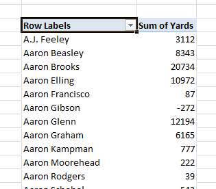
So far I have just been adding the Yards field to my reports, yielding a Sum of Yards column:

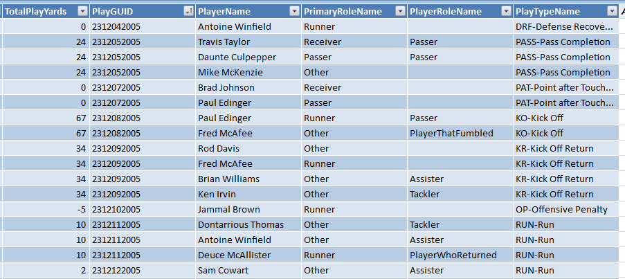
But my source table (the Plays table) typically contains multiple records for a single play, with each record detailing a different player involved in the play, and their role. Check THIS out:

Um… yeah. There are a multiple rows per play AND a bajillion types of plays. And they are all mixed in there in one table. Scanning the screenshot above and applying my knowledge of football, I can say that only ONE row should actually count toward Rushing Yards.
I believe the technical database schema term for this sort of thing is “icky.” But I don’t think we can blame anyone for this. Really, football is pretty complex – for a given event, the amount of data that we want to capture can vary tremendously, simply based on what type of play it was, and even based on what HAPPENED on the play.
That’s pretty complex. But PowerPivot has a secret weapon for this sort of thing.
Und now’s the time on Sprockets when we Calculate!
In traditional Excel, I would solve this problem like this: I’d create a new column in the Plays table, name it [Rushing Yards], and then use =IF() to give that column a value only when it indeed supposed to count as Rushing Yards. Then I’d add the Sum of that column to my Pivot.
But as I repeat that process for every other type of yardage – passing, receiving, etc., I’m going to make an already unwieldy table even larger, which makes my life harder (more scrolling) AND increases file size.
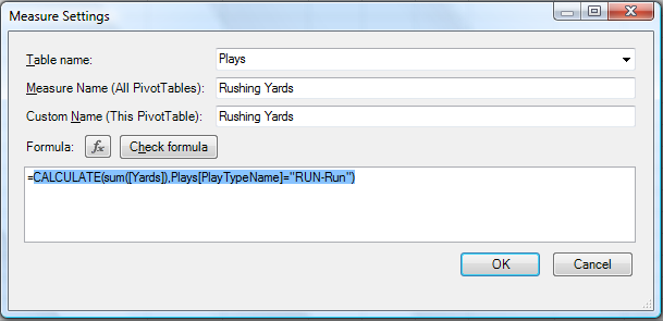
In PowerPivot, I don’t have to do that. I just go straight to the Pivot Table itself and add a new DAX measure:

Let’s zoom in on that formula:

That’s pretty simple. The first param is the numerical quantity you are trying to measure – Sum of Yards in this case. All subsequent parameters are filters/conditions that you want to apply while evaluating that quantity. Which in this case, is Play Type = “RUN-run”
In the next post, I’ll tell you whether that works 🙂 And explain in more detail what’s going on here. If my voice is feeling better, I will do it as a video. But for now the quiet masses who prefer text and pics may rejoice 🙂
Get in touch with a P3 team member