I often have inputs I know today and want to “run them out” into the future applying certain parameters along the way to create a projection. I’m in finance, so my needs will almost always have a financial planning bias, but there’s no reason why this wouldn’t have general mathematical, statistical, or scientific utility as well. Heck, I’ve gleaned lots from non-financial posts and applied them to my work. Inputs could be virtually anything in this DAX pattern. If you use a bottom-up approach to financial planning and analysis (FP&A), it should be especially easy to relate to this post. To keep things relatively straightforward, I’ll show you how to produce a labor cost projection using a project start date, hourly rate, and employee start and end dates.
Please click here to download the workbook to follow along.
First, the setup.
I created three tables in my “data model” (using quotes here because the tables are disconnected). I won’t spend too much time talking about getting data into the data model; however, I have been experimenting and becoming more comfortable with Power Query. Some P3 Adaptive guru—maybe Ryan Sullivan—recently gave me a pointed piece of advice: “If you can put it in Power Query, do it.” Even though Power Query has been out of my comfort zone, after receiving this advice, I decided it was time to get uncomfortable. Boy, has it paid off!
Here’s a summary of what I did to set up these three tables:
Calendar: used List.Dates and set parameters to create a one-year table. In my work, which involves lots of projects, I use an approach I learned from Ken Puls’ blog to create a dynamic parameter so I can change the start/end dates of the projects and Power Query makes a table between those exact dates. It’s awesome.
Project Start Date: Excel table sucked into the data model via Power Query.
Data Input: Excel table sucked into the data model via Power Query.
So, I lied. I’m breaking the “if you can put it into Power Query, do it” rule in the name of connecting with you more on DAX calculated columns than M, which is beyond where I want to go with this post. In my calendar table, I created the following columns:
Day Number of Week: =
WEEKDAY ( [Date] )
Work Day: =
SWITCH ( [Day Number of Week], 1, 0, 7, 0, 1 )
Month: =
MONTH ( [Date] )
Year: =
YEAR ( [Date] )
Year Month: =
[Year] & “-“
& [Month]
Year Month Sort: =
( [Year] * 100 )
+ [Month]
The combination of “Day Number of Week” and “Work Day” gives me similar functionality to NETWORKDAYS in Excel, so I’m able to determine the exact number of work days per month. My company works in the Middle East where weekends fall on Fri/Sat instead of Sat/Sun, which has an impact on the number of workdays. In addition to giving me the NETWORKDAYS functionality, it also gives me the opportunity to move my workable days around to accommodate different schedules.
The rest of the calculated columns are not part of the pattern per se; they’re just part of my “visualization” requirements. I’ll leave you to your own. There is no shortage of information how to create calendar tables, here is just one Matt Allington penned that I often reference.
For project start date, I just need the date in a measure, so I use:
Project Start Date :=
MAX ( [Value] )
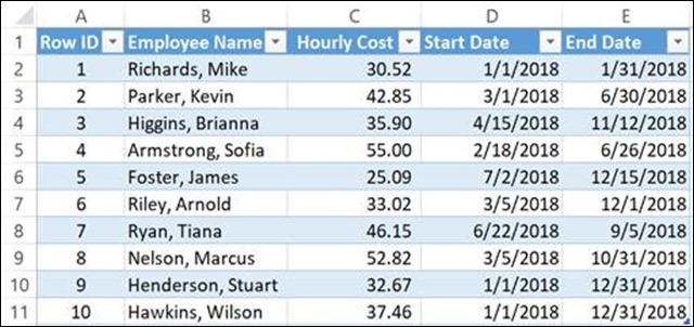
Finally, on the data input tab, I’ve created a table with a row ID (because every good table has a row ID—you’ll never know when you’ll need it!), employee name, hourly rate, and the start and end dates of the employee’s engagement on this project. I’ve given you a variety of start an end dates (i.e., duration and start/end times within a month) to show you the accuracy of this pattern.
Here is a look at that data input table:
Second, calculating the projection.
I’ll list the three measures that make this calculation work and then go into detail on the other side:
1. Num of Working Days :=
CALCULATE (
SUMX ( ‘Calendar’, ‘Calendar'[Work Day] ),
FILTER (
‘Calendar’,
‘Calendar'[Date] >= MAX ( DataInput[Start Date] )
&& ‘Calendar'[Date] <= MAX ( DataInput[End Date] )
)
)
2. Total Working Days :=
CALCULATE ( SUMX ( DataInput, [Num of Working Days] ) )
3. Labor Cost :=
CALCULATE (
SUMX ( DataInput, DataInput[Hourly Cost] * 8 * [Total Working Days] )
)
The first measure calculates the number of working days. The second iterates the result of #1 over the DataInput table and is also the measure used in our first report, which shows total days worked.
The third measure calculates the total cost using the hour cost multiplying by an eight-hour day and the total working days calculated in #2. “Labor Cost” is the measure used in our second report.
Where you can go from here…
I’ve given you the basic pattern; the application of it is only limited by your imagination. I’ve used this to calculate labor cost as above, apply a revenue calculation (or gross margin %), and utilize it within my first post to create a project forecast (i.e., ITD invoiced plus projection vs. project budget). I’ve also used this to take a lump sum amounts—say revenue forecasts from various streams and forecast—to project them out over time to better understand how we might collect on it in the future. Finally, I’ve used this as a calculator on the fly answering the question: “if I know X, Y, and Z, I wonder how that will look over time?” My answer to that: “Wait a sec.” Usually, it’s a dataset with hundreds of lines of inputs, so it makes any other way of calculating a result quickly pale in comparison.
Forget bending spoons with your mind – there’s no money in it.
It takes a special kind of mindset to “bend” data (and software!) to the human will. As this article demonstrates, we at P3 Adaptive can twist Power BI into a pretzel if that’s what an organization needs. (A robust, trustworthy, industrial-strength pretzel of course).
The data-oriented challenges facing your business require BOTH a nimble toolset like Power BI AND a nimble mindset to go with it. And as Val Kilmer / Doc Holladay once said, we’re your huckleberry.


