Data intelligence that gives you a competitive edge
P3 Adaptive brings business leaders the action-ready insights that propel you forward, with none of the B.S. that slows you down.

We've created over a billion dollars in value for our clients.
We take your disparate, noisy, chaotic data and distill it down to simple dashboards which help you spot problems and opportunities. We empower companies to take decisive action and constantly improve.


We measure iterations in minutes, not months.
Our best-in-class services:
Advisory Services
Transform your org by getting an expert perspective on analytics tools and trends.
Learn More


P3 Adaptive has empowered us, rather than making us dependent on them. Just the right amount of education, direction, and smart help, whenever we need it. The results have been transformational.
MIKE MISKELL, DIRECTOR OF PROCESS IMPROVEMENT @ KAMAN INDUSTRIAL TECHNOLOGIESSome outcomes we can bring you:
Org-Wide Alignment
Get your entire org pulling in one direction and flow top-level goals down the orgchart with smart scorecards.
Optimized Pricing
Confidently apply profit-maximizing pricing plans, tuned by segment, based on detailed elasticity analysis.
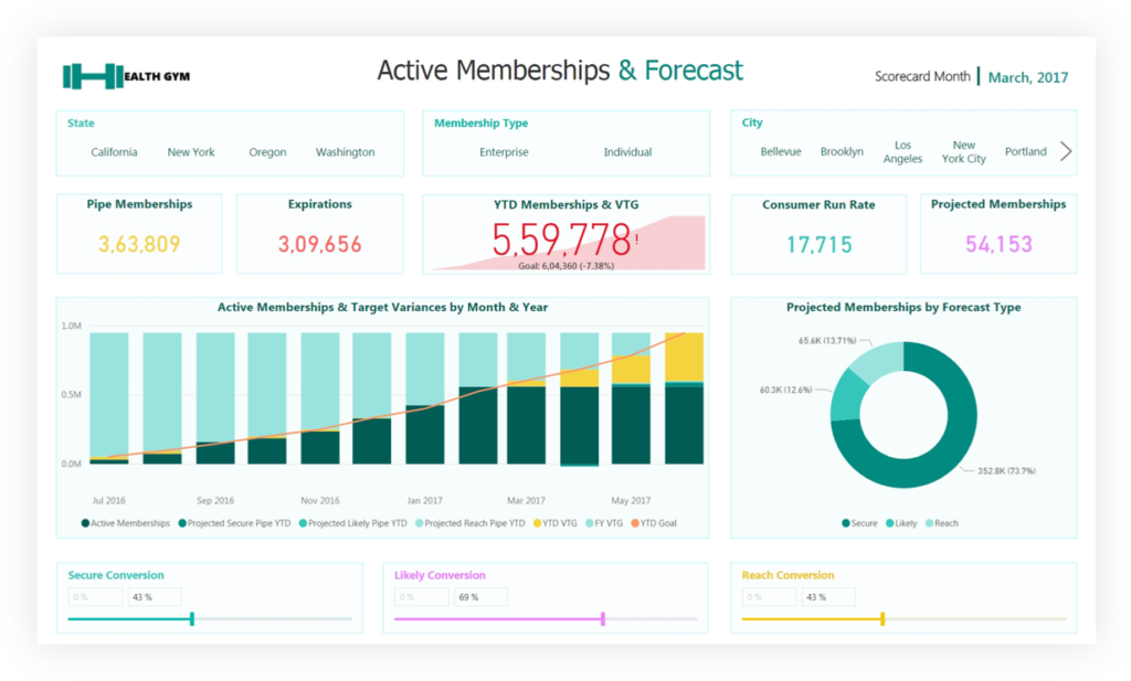
Precision Forecasting
Paint a confident baseline picture of the future based on known data, then create & evaluate scenarios for the unknowns.
Streamlined Budgeting & Planning
Integrate planning, budgeting, and reporting into a single environment. No spreadsheets, no versioning hell.
Comprehensive Sales Reporting
Bring all revenue data to your fingertips. Quickly compare across all sales channels & business segments.
Supply Chain Optimization
Have the right amount of inventory in the right place, at the right time, for the right price - always. No fire drills.
Cross-Silo Visibility
Your business runs on a mix of systems, but you get end-to-end insight in one place - with no expensive infrastructure.
Accounting and Finance Agility
From daily reporting to end-of-period statements & audits, we take your processes from weeks down to hours.
Data-Driven Culture Change
The transition from "old school" to modern & data-driven is easier than you think. We help you lead by example.
Real-Time Steering
Monthly & quarterly reports can now be run weekly or daily - so you can make adjustments before it's too late.
Optimized Digital Marketing
Customized dashboards integrating your CRM and in-house data paint a complete picture you can't get from ad portals.
Technology Cost Savings
High-priced specialty software & services are routinely replaced by proper utilization of your Microsoft subscription.
Bringing business savvy to BI problems.


Narayana Windenberger
Narayana (pronounced “Na-ryan-a," or "Nar" for short) years ago began using Power BI as an antidote to the crippling turnaround times of traditional BI. His MBA background firmly grounds him in business, but his considerable technical skills define our view of the future: one led by a new breed of hybrid IT/Business operators.
About UsNarayana (pronounced “Na-ryan-a," or "Nar" for short) years ago began using Power BI as an antidote to the crippling turnaround times of traditional BI. His MBA background firmly grounds him in business, but his considerable technical skills define our view of the future: one led by a new breed of hybrid IT/Business operators.
About UsUnfiltered Wisdom
Each week we speak with business leaders, executives and other industry professionals to bring you the stories of the people behind the data. New episodes of the Raw Data by P3 Adaptive podcast drop every Tuesday.